erucakra: A Physically-Motivated Toy Model for Climate Tipping Point Dynamics

A three-variable dynamical system model exhibiting bifurcation behavior for analyzing climate tipping points under IPCC AR6 SSP scenarios.

Model Description

The model describes climate system dynamics through a coupled ordinary differential equation system:

dx/dt = y
dy/dt = x(z - z_crit - x²) - cy
dz/dt = ε(A(t)/A_scale - z - βx²)

Physical Interpretation

Variable	Description	Physical Analog
x	Fast climate variability	Interannual oscillations (ENSO-like modes)
y	Rate of change of x	Momentum in phase space
z	Slow accumulated forcing	Ocean heat content, ice sheet mass proxy
A(t)	External forcing	Radiative forcing (W/m²) from SSP scenarios

Bifurcation Dynamics

The system undergoes a supercritical pitchfork bifurcation when z crosses z_crit:

• z < z_crit: Single stable equilibrium at x = 0 (stable climate)
• z > z_crit: Bistable regime with equilibria at x = ±√(z - z_crit) (tipped state)

The effective potential governing the fast dynamics:

V(x) = -x²(z - z_crit)/2 + x⁴/4

This creates a double-well potential after tipping, representing irreversible regime shifts.

Parameters

Symbol	Description	Default	Typical Range
c	Damping coefficient	0.2	0.1 – 0.5
ε	Timescale separation (slow/fast)	0.02	0.01 – 0.05
β	Feedback strength (variability → accumulation)	0.8	0.5 – 1.5
z_crit	Critical tipping threshold	0.55	0.3 – 0.8
A_scale	Global forcing normalization	13.0 W/m²	—

Normalization Strategy

All scenarios use a global normalization scale (A_scale = 13.0 W/m²) based on the SSP5-8.5 peak forcing. This ensures consistent comparison across scenarios:

Scenario	Peak Forcing	Normalized Peak
SSP1-2.6	~3.6 W/m²	0.28
SSP2-4.5	~5.6 W/m²	0.43
SSP3-7.0	~11.6 W/m²	0.89
SSP5-8.5	~13.2 W/m²	1.02

Installation

From PyPI

pip install erucakra

From Source

git clone https://github.com/sandyherho/erucakra.git
cd erucakra
pip install poetry
poetry install

Usage

Command Line Interface

Run a single scenario:

erucakra run --scenario ssp245

Run all scenarios:

erucakra run --all-scenarios

Adjust tipping sensitivity:

# Lower z_crit = more sensitive (tips earlier)
erucakra run --scenario ssp245 --z-crit 0.4

# Higher z_crit = less sensitive (tips later)
erucakra run --scenario ssp370 --z-crit 0.7

Use custom forcing data:

erucakra run --forcing ./my_forcing.csv

Use a configuration file:

erucakra run --config ./configs/custom.yaml

List available scenarios:

erucakra list

Run sensitivity analysis:

erucakra sensitivity --scenario ssp245 --z-crit-min 0.3 --z-crit-max 0.8 --n-samples 10

Python API

from erucakra import ClimateModel, GLOBAL_A_SCALE, DEFAULT_Z_CRIT_ABSOLUTE

# Initialize model with default parameters
model = ClimateModel(
    c=0.2,           # damping
    epsilon=0.02,    # timescale separation
    beta=0.8,        # feedback strength
    z_crit=0.55,     # absolute tipping threshold
)

# Run simulation
results = model.run(
    scenario="ssp370",
    t_end=600.0,
    add_noise=True,
)

# Check results
print(f"Scenario: {results.scenario_info['name']}")
print(f"Tipped: {results.tipped}")
print(f"Max z: {results.max_z:.3f}")
print(f"z_crit: {results.z_crit:.3f}")
print(f"First crossing: Year {results.first_crossing_year}")

# Export outputs
results.to_csv("output.csv")
results.to_netcdf("output.nc")
results.to_png("timeseries.png")
results.to_gif("phase_space.gif")

Analyzing Multiple Scenarios

from erucakra import ClimateModel, SCENARIOS

model = ClimateModel()

for scenario_key in SCENARIOS:
    results = model.run(scenario=scenario_key, add_noise=False)
    summary = results.summary()
    
    print(f"{scenario_key}: "
          f"max_z={summary['max_z']:.3f}, "
          f"tipped={summary['tipped']}, "
          f"crossing={summary['first_crossing_year']}")

Custom Forcing Data

Forcing CSV format:

time,forcing
1750,0.3
1850,0.5
2000,2.5
2100,5.5
2200,4.0

from erucakra import ClimateModel
from erucakra.io import load_forcing_csv

# Load custom forcing
times, values = load_forcing_csv("my_forcing.csv")

# Run with custom forcing
model = ClimateModel(z_crit=0.5)
results = model.run(
    forcing=values,
    forcing_times=times,
    t_end=600.0,
)

Sensitivity Analysis

from erucakra import ClimateModel

model = ClimateModel()

# Vary z_crit to find critical threshold
results_list = model.sensitivity_analysis(
    scenario="ssp245",
    z_crit_range=(0.3, 0.6),
    n_samples=10,
    add_noise=False,
)

for z_crit, results in results_list:
    if results:
        print(f"z_crit={z_crit:.2f}: tipped={results.tipped}, max_z={results.max_z:.3f}")

Available Scenarios

Scenario	Description	Peak Forcing
ssp126	SSP1-2.6 Sustainability	~3.6 W/m²
ssp245	SSP2-4.5 Middle Road	~5.6 W/m²
ssp370	SSP3-7.0 Regional Rivalry	~11.6 W/m²
ssp585	SSP5-8.5 Fossil Development	~13.2 W/m²

Output Formats

Format	Description
CSV	Full data table with all variables and diagnostics
NetCDF	CF-compliant NetCDF4 with compression and metadata
PNG	Time series diagnostic plot with threshold indication
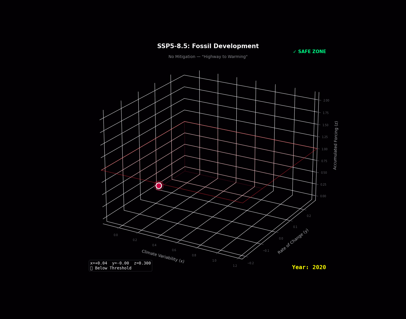
GIF	Animated 3D phase space visualization

Output Variables

Variable	Units	Description
year	year	Calendar year (integer)
year_decimal	year	Decimal year (fractional)
x_variability	—	Fast climate variability
y_momentum	1/time	Rate of change
z_accumulated	—	Slow accumulated state
A_forcing_Wm2	W/m²	Radiative forcing
A_normalized	—	Normalized forcing (A/A_scale)
warming_proxy_celsius	°C	Approximate temperature anomaly
distance_to_threshold	—	z - z_crit
regime	—	"tipped" or "not_tipped"

Configuration

Create a custom configuration file:

# my_config.yaml
model:
  damping: 0.2
  epsilon: 0.02
  beta: 0.8
  z_crit: 0.55  # Absolute threshold

simulation:
  t_start: 0.0
  t_end: 600.0
  n_points: 48000
  add_noise: true
  noise_level: 0.03

outputs:
  formats:
    - csv
    - netcdf
    - png
    - gif
  base_dir: ./outputs

Run with configuration:

erucakra run --config my_config.yaml --scenario ssp370

Mathematical Details

Fast Subsystem (x, y)

The (x, y) subsystem forms a damped Duffing-type oscillator:

d²x/dt² + c(dx/dt) = x(z - z_crit) - x³

The cubic term -x³ provides saturation, preventing unbounded growth.

Slow Subsystem (z)

The z equation is a forced relaxation:

dz/dt = ε(A_normalized - z - βx²)

At quasi-equilibrium: z_eq ≈ A_normalized - βx²

The βx² term creates hysteresis: oscillations reduce effective forcing, so tipping may not reverse when forcing decreases.

Fixed Points

For the full system at equilibrium:

Pre-tipping (z < z_crit):

• Single stable fixed point: (x, y, z) = (0, 0, A_normalized)

Post-tipping (z > z_crit):

• Unstable: (0, 0, z_eq)
• Stable: (±√(z - z_crit), 0, z_eq)

where z_eq satisfies the implicit equation from the feedback.

Citation

If you use this model in your research, please cite:

@software{erucakra2025,
  author = {Herho, Sandy H. S.},
  title = {\texttt{erucakra}: {A} {P}hysically-{M}otivated {T}oy {M}odel for {C}limate {T}ipping {P}oint {D}ynamics},
  year = {2025},
  url = {https://github.com/sandyherho/erucakra},
  version = {0.0.1}
}

License

MIT License © 2025 Sandy H. S. Herho