pygidSIM

pygidSIM calculates GIWAXS patterns from CIF files or other crystal structure descriptions.

Installation

Install from PyPi

pip install pygidsim

Install from source

First, clone the repository:

git clone https://github.com/mlgid-project/pygidSIM.git

Then, to install all required modules, navigate to the cloned directory and execute:

cd pygidSIM
pip install -e .

Development Installation

For development and testing, install with development dependencies:

pip install -e .[dev]

Testing

The project uses pytest for testing. To run the test suite:

# Run all tests
pytest

# Run tests with coverage report
pytest --cov=pygidsim --cov-report=html

# Run tests in parallel
pytest -n auto

Usage

From CIF

To calculate the peak positions and their intensities in 2D GIWAXS pattern (q_xy, q_z) from a CIF file with the default orientation hkl = [001] (vector normal to the substrate, i.e. {001} contact plane) run the following:

from pygidsim.experiment import ExpParameters
from pygidsim.giwaxs_sim import GIWAXSFromCif

params = ExpParameters(
    q_xy_range=(0, 2.7),
    q_z_range=(0, 2.7),
    en=18000
)  # experimental parameters
el = GIWAXSFromCif(path_to_cif, params)
q_2d, intensity = el.giwaxs.giwaxs_sim()  # q_2d is array with shape (2, peaks number)

To add a crystal rotation use the argument orientation with the value "random" or a numpy array containing the corresponding Miller indices [hkl]:

q_2d, intensity = el.giwaxs.giwaxs_sim(orientation='random')

q_2d, intensity = el.giwaxs.giwaxs_sim(orientation=numpy.array([2., 0., 1.]))

For 3D powder diffraction simulation (non-oriented case) use orientation=None:

q_1d, intensity_1d = el.giwaxs.giwaxs_sim(orientation=None)

To return the Miller indices, you can use the argument return_mi = True:

q_2d, intensity, mi = el.giwaxs.giwaxs_sim(return_mi=True)

To restrict the maximum Miller index for simulation use the argument max_mi:

q_2d, intensity = el.giwaxs.giwaxs_sim(max_mi=3)

Crystal description

To calculate a GIWAXS pattern from your own description, use the following example:

import numpy as np
from pygidsim.giwaxs_sim import GIWAXS, Crystal

# space group number
spgr = 221  # alternatively, use e.g. '146:R'

# lattice parameters [a, b, c, α, β, γ]
lat_par = np.array([6.3026, 6.3026, 6.3026, 90., 90., 90.], dtype=np.float32)

# list of atoms
atoms = np.array(['Pb', 'I', 'I', 'I', 'N'])

# relative atom positions
atom_positions = np.array(
    [[0., 0., 0.],
     [0.5, 0., 0.],
     [0., 0.5, 0.],
     [0., 0., 0.5],
     [0.5, 0.5, 0.5]], dtype=np.float32
)

# occupancies of the corresponding sites
occupancy = np.array([1., 1., 1., 1., 1.], dtype=np.float32)

cr = Crystal(lat_par, spgr, atoms, atom_positions, occupancy)
el = GIWAXS(cr, params)
q_2d, intensity = el.giwaxs_sim(orientation='random')

The intensities are set to one in case the arguments atoms or/and atom_positions are not provided.

Visualization

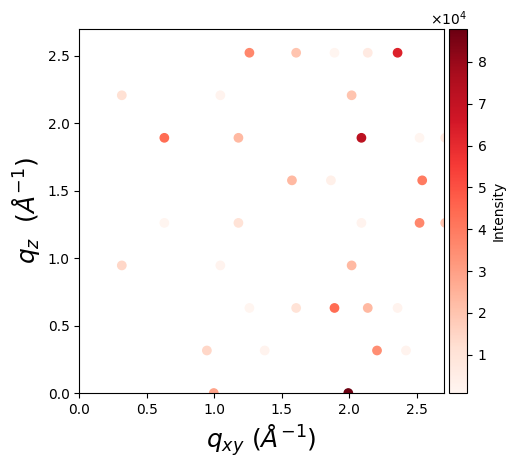
One can visualize a GIWAXS pattern using matplotlib:

import matplotlib.pyplot as plt
from mpl_toolkits.axes_grid1.axes_divider import make_axes_locatable

fig, ax = plt.subplots(figsize=(5, 5))
ax.set_aspect('equal')
scatter = ax.scatter(*q_2d, c=intensity, cmap='Reds')

ax.set_xlabel(r'$q_{xy}$ $(Å^{-1})$', fontsize=18)
ax.set_ylabel(r'$q_{z}$ $(Å^{-1})$', fontsize=18)

divider = make_axes_locatable(ax)

# Append a new axes for the color bar to the right of the current axes
cax = divider.append_axes("right", size="5%", pad=0.05)

# Create color bar in the new axes
colorbar = fig.colorbar(scatter, cax=cax)
colorbar.set_label('Intensity')

plt.show()

Citation

If you use this package in your research, please cite it as follows:

Romodin, M., Starostin, V., Lapkin, D., Hinderhofer, A., & Schreiber, F. (2025).
mlgid-project/pygidSIM: v0.1.1. Zenodo. https://doi.org/10.5281/zenodo.17609569