This is some raw and unedited content that was originally targeting Chapter 11 of the Vision Language Models book. As we won't manage to fit this in the book, we decided to make it publicly available here. We hope you find this useful

❤️ Merve, Miquel, Andi and Orr.

Hands on toolkit

Are you ready to get hands on with robots? Before diving into inference and training, let's get oriented with the tools you will use.

Isaac Sim

Isaac Sim is NVIDIA's robotics simulation platform, and it serves two critical roles in VLA development. First, it's where you will run inference to see trained models in action. You can load a policy, spawn a simulated robot, and watch it attempt tasks in a physics-accurate environment. This is invaluable for evaluation: you can run hundreds of episodes overnight without wearing out motors or breaking objects. Second, Isaac Sim is where you will record teleoperated demonstrations. You control a virtual robot through a task, and the system captures synchronized camera feeds, joint states, and actions: exactly the data format you need for training.

While Isaac Sim can run locally if you have a capable NVIDIA GPU, the hardware requirements are substantial. To prepare this chapter we used a cloud instance together with a set of containers that we prepared for you (see prerequisites and setup section).

Within Isaac Sim, you will use two key components:

1. LeIsaac: the bridge between Isaac Sim and the LeRobot ecosystem. It provides teleoperation interfaces for recording demonstrations, handles the conversion of Isaac's internal state to the observation format VLAs expect, and manages episode recording to HDF5 files. When you teleoperate a robot in Isaac Sim, LeIsaac is what captures those multi-camera RGB streams, joint positions, and gripper states into a synchronized dataset.
2. GR00T tooling to run model inference within Isaac Sim using a client-server architecture. You start an inference server that loads the model weights and handles the GPU-intensive action generation. A separate client connects to your Isaac Sim environment, feeds observations to the server, receives action chunks back, and executes them on the simulated robot. This separation mirrors real-world deployment patterns: your policy runs on a GPU workstation while the robot controller handles low-level execution. Learning this architecture in simulation means you already understand the deployment model when you move to physical hardware.

LeRobot

LeRobot is a library from Hugging Face that brings order to the chaos of robot learning datasets. Every research group historically had their own data format, their own normalization schemes, their own training scripts. LeRobot provides a standardized dataset format that works across different robots and tasks, pre-built data loaders that handle normalization and batching correctly, and a lerobot-train CLI that abstracts away the training loop boilerplate.

The practical benefit is interoperability. Once your demonstrations are in LeRobot format, you can train any compatible policy architecture without rewriting data pipelines. You can share datasets on Hugging Face Hub and use datasets others have shared.

LeRobot’s SO-100

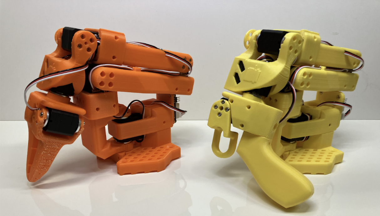
The SO-100 is a low-cost robot arm designed specifically for the LeRobot ecosystem. What makes it particularly useful for VLA development is its leader-follower configuration: instead of fighting with a gamepad or keyboard to control a robot through a task, you simply guide the leader arm through the motions you want. The follower arm replicates these movements while cameras and encoders record everything.

You just saw how useful the SO-100 can be for data collection. Once you've trained a policy, you can run inference on the follower arm directly. The model receives camera observations, generates actions, and the follower executes them. If you don’t have a follower arm, you can record demonstrations of a real task and use those trajectories to validate that your Isaac Sim environment behaves similarly. Conversely, policies trained partly in simulation can be fine-tuned on real SO-100 data to bridge the sim-to-real gap.

For this chapter, physical hardware is optional. Everything in the hands-on tracks works entirely in simulation. But if you have access to an SO-100 or similar setup, you'll find that the skills transfer directly: the data formats are the same, the training pipelines are the same, and the evaluation metrics mean the same thing. The main addition is respecting that real robots can break things (including themselves) so you approach deployment more carefully.

Prerequisites and Setup

Before diving into the hands-on tracks, let's get the environment running. We have prepared a repository that bundles Isaac Lab, the GR00T inference server, LeIsaac, and a web-based VS Code environment so you can focus on robotics.

You will need a Linux host with Docker installed, an NVIDIA GPU with recent drivers (we tested the setup on L40S).

Start by cloning the repository:

sudo apt-get install git-lfs  
git lfs install  
git clone [https://github.com/mfarre/chapter-11-vla.git](https://github.com/mfarre/chapter-11-vla.git)

Now, you can build and launch the stack:

cd chapter-11-vla/isaac-launchable/isaac-lab/  
docker compose up

As you can see in the next figure, this brings up several containers working together:

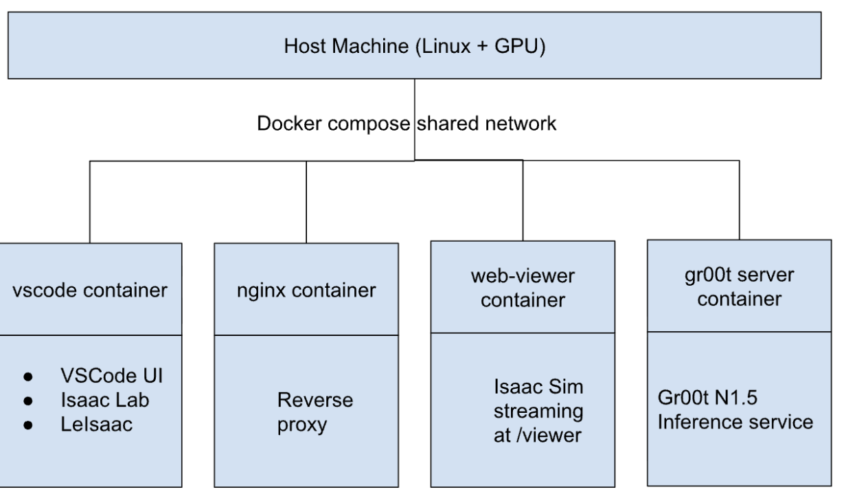
All containers share the host network. When LeIsaac (running inside the vscode container) needs to query GR00T for actions, it simply connects to localhost:6006. To view the simulation, you open <your host>:80/viewer in your browser. This mirrors real deployment patterns where the policy server and robot controller are separate processes that communicate over the network.

Once the containers are running, open your browser to port 80 to access the VS Code server. You will do all your work from this web-based IDE, which has direct access to Isaac Lab, LeIsaac, and can reach the GR00T server.

Inside the VS Code terminal, install the LeIsaac package and its dependencies:

cd /workspace/leisaac/  
pip install -e source/leisaac  
pip install pyzmq  

You are now ready for both hands-on tracks.

GR00T N1.5 on Isaac Lab

In this section, you will run GR00T N1.5 in Isaac Lab and observe how a pre-trained model handles a manipulation task without any fine-tuning on your specific environment. Your goal is to get the environment running (sounds easy but it takes some effort), see the robot move, and build intuition for how action chunks, language conditioning, and inference latency affect real behavior.

Running Inference

From the VS Code terminal, launch the policy inference script:

cd /workspace/leisaac

python scripts/evaluation/policy_inference.py \  
  --task=LeIsaac-SO101-PickOrange-v0 \  
  --policy_type=gr00tn1.5 \  
  --policy_host=localhost \  
  --policy_port=6006 \  
  --policy_timeout_ms=5000 \  
  --policy_action_horizon=16 \  
  --policy_language_instruction="pick up the orange and place it on the plate" \  
  --device=cuda \  
  --enable_cameras \ 
  --kit_args="--no-window --enable omni.kit.livestream.webrtc"  

Open localhost:80/viewer in your browser to watch the simulation. It should look like something similar to Figure 11-5.

Watch the logs as the system initializes. You will see Isaac Lab describe the environment setup: observation spaces, action spaces, termination conditions. Then evaluation begins: [Evaluation] Evaluating episode 1... followed by the robot actually attempting to pick up the oranges and place it on the plate.

Take a moment to observe the robot's behavior. Notice how movements are smooth rather than jerky: this is the action chunking at work. The model predicts 16 future actions at once (that's what --policy_action_horizon=16 means), and the robot executes them sequentially while the next chunk is being generated. You are watching the asynchronous control pattern from Section 11.2.1 in action.

Experimenting with the Knobs

Running inference once shows you that the system works. Running it with different parameters teaches you how it works. The following experiments are safe to try and will build your intuition for VLA behavior.

Action horizon. The --policy_action_horizon parameter controls how many future actions GR00T predicts per inference call. This is the chunk size we discussed earlier, and it directly affects the character of robot motion.

Try running with different values:

# Short horizon - more reactive*  
--policy_action_horizon=4  
# Medium horizon (default)*  
--policy_action_horizon=16  
# Long horizon - smoother, more committed*  
--policy_action_horizon=32  

With short horizons, the robot re-plans frequently. You may notice more reactive behavior but also potential jitter as each new plan slightly disagrees with the previous one. With long horizons, movements become smoother: the robot commits to a trajectory and follows through. All comes at a cost my friend: if something unexpected happens mid-chunk, the robot can't react until the current chunk finishes executing.

This tradeoff between reactivity and smoothness is fundamental to action-chunk policies. There is no universally correct answer: it depends on your task. As you can imagine, fast changing environments need shorter chunks and predictable tasks benefit from longer ones.

Language instruction. GR00T is conditioned on natural language, which means you can change what the robot attempts by changing the instruction. Try different phrasings:

--policy_language_instruction="move the orange to the plate"  
--policy_language_instruction="put the citrus fruit on the dish"
--policy_language_instruction="pick the orange and hold it in the air"  

Some variations will work fine: the model has learned that "move," "put," and "place" can mean similar things in manipulation contexts. Others might produce strange behavior. "Hold it in the air" describes a different end state than placing on the plate; does the model handle this? "Citrus fruit" and "dish" are synonyms that the model may or may not have seen during training.

Pay attention to where language grounding breaks down. When the robot behaves unexpectedly, ask yourself: is this a perception failure (it can't find the "citrus fruit"), a semantic failure (it doesn't know "dish" means plate), or a behavior failure (it knows what you want but can't execute it)? These distinctions matter when you're debugging real deployments.

Timeout and latency. The --policy_timeout_ms parameter sets how long the client waits for the server to return actions before giving up. This is your window into the inference latency budget.

Try lowering it:

--policy_timeout_ms=1000  

If your GPU is under load or the model is large, you might start seeing timeout errors. The robot pauses, waiting for actions that arrive too late. This is what happens in real systems when inference can't keep up with control frequency—the action queue runs dry and the robot stalls.

Raise it to see the opposite extreme:

--policy_timeout_ms=10000  

Now you will wait a long time before a slow inference is declared a failure. This is safer in that you get fewer timeouts, but it also means problems take longer to surface. In a real deployment, you would tune this based on your actual inference latency distribution: tight enough to catch real problems quickly, loose enough to handle normal variation.

These three knobs that we have seen (action horizon, language instruction, and timeout) give you direct access to the core tradeoffs in VLA deployment. Spend some time experimenting before moving on to develop your intuition.

Data Gathering and Fine-Tuning SmolVLA

Foundation models are impressive, but eventually you need a policy tuned to your specific task and environment. This section walks you through the complete pipeline: recording teleoperated demonstrations in Isaac Lab, converting them to LeRobot format, and fine-tuning SmolVLA on your data.

Step 1: Record Demonstrations

High-quality demonstrations are the foundation of imitation learning. The model can only learn behaviors that exist in your data, so the time you invest here pays dividends throughout training.

From the VS Code terminal, launch the teleoperation script:

cd /workspace/leisaac

python scripts/environments/teleoperation/teleop\_se3\_agent.py \ 
  --task=LeIsaac-SO101-PickOrange-v0 \  
  --teleop\_device=keyboard \  
  --num\_envs=1 \  
  --device=cuda \  
  --enable\_cameras \  
  --record \  
  --dataset\_file=./datasets/pick\_orange\_demos.hdf5 \  
  --kit\_args="--no-window \--enable omni.kit.livestream.webrtc"  

Open localhost:80/viewer in your browser to see the simulation. You'll control the robot using your keyboard with the controls on the table below. Do not worry, the first minutes it is difficult for everybody to control the robot with the keyboard.

Movement Controls	Forward / Backward	W / S
	Left / Right	A / D
	Up / Down	Q / E
Rotation Controls	Rotate (Yaw) Left / Right	J / L
	Rotate (Pitch) Up / Down	K / I
Gripper	Open / Close	U / O

SO-100 Keyboard controls

The recording workflow goes like this:

• Click into the Isaac window and press B to begin teleoperation
• Your keyboard inputs now drive the robot and get recorded into the HDF5 file. Guide the robot through the task: move to the orange, close the gripper, lift, carry to the plate, release
• When you have completed a good demonstration, press N to mark it as successful and reset the scene. If you mess up mid-demonstration, press R to mark it as a failure and reset. Either way, you're back at the starting state and can press B to begin the next episode.

A typical recording session looks like: B -> teleoperate -> N (success) -> B -> teleoperate -> R (messed up) -> B -> teleoperate -> N -> ... repeat until you have enough data. When you're done, Ctrl-C in the terminal ends the session and all episodes went into the HDF5 file that we specified.

How many demonstrations do you need? For a simple task like picking and placing a single object, 30-50 good demonstrations are a reasonable starting point. More is better, but you will see meaningful learning even with modest amounts of data. Quality matters more than quantity: ten clean demonstrations teach more than fifty sloppy ones.

Variation is essential if you always pick up the orange from the same position, your policy learns to reach for that exact spot and fails when deployment conditions differ by a few centimeters. Vary your demonstrations: approach from different angles, pick up the orange when it's in different positions, and place it on different parts of the plate.

Step 2: Convert to LeRobot Format

The HDF5 file from Isaac Lab needs to be converted to LeRobot's standardized format before training. We'll do this on the host machine rather than inside the container, since you'll also run training there.

First, set up a conda environment with LeRobot and SmolVLA support. We do this directly in our host machine

# If you don't have conda installed  
wget https://repo.anaconda.com/miniconda/Miniconda3-latest-Linux-x86_64.sh  
bash Miniconda3-latest-Linux-x86_64.sh  
source ~/.bashrc

# Create the environment*  
conda create -n lerobot python=3.10  
conda activate lerobot

# Install LeRobot with SmolVLA support*  
pip install "lerobot[smolvla]"  
pip install h5py

sudo apt-get install -y ffmpeg libavcodec58 libavutil56 libavformat58  

Copy your recorded demonstrations from the Docker container to the host:

docker cp vscode:/workspace/leisaac/datasets/pick_orange_demos.hdf5 \\
  ./datasets/dataset.hdf5  

Run the conversion script:

cp chapter-11-vla/leisaac/scripts/convert/isaaclab2lerobot\_updated.py .

python isaaclab2lerobot\_updated.py  

The script converts your HDF5 recordings into LeRobot's format, handling the camera key mapping, action normalization, and metadata extraction. By default, it creates a dataset in your HuggingFace cache at local/so101_test_orange_pick. You can edit the script if you want a different name.

Step 3: Fine-Tune SmolVLA

You are ready to train. SmolVLA's compact size makes it practical to fine-tune on a single consumer GPU.

export TOKENIZERS\_PARALLELISM=false

lerobot-train \ 
  --policy.type smolvla \
  --policy.pretrained_path lerobot/smolvla_base \  
  --dataset.root ~/.cache/huggingface/lerobot/local/so101_test_orange_pick \  
  --dataset.repo_id local/test \  
  --output_dir outputs/train/my_smolvla \  
  --job_name my_smolvla_training \  
  --batch_size 64 \  
  --steps 20000 \  
  --policy.optimizer_lr 1e-4 \  
  --policy.device cuda \  
  --policy.push_to_hub false \  
  --save_checkpoint true \  
  --save_freq 5000 \
  --log_freq 100  

Tuning for your setup. The configuration above works well for a dataset of 50-100 episodes on a GPU with 24GB of VRAM. You may need to adjust based on your situation:

Some rules of thumb:

• For training steps, scale roughly with your data: 50 episodes warrant 10-20K steps, 200 episodes can support 20-40K steps. Taking more steps with little data just leads to overfitting.
• If you hit CUDA out-of-memory errors, reduce batch size to 32 or 16. You can also enable gradient checkpointing if available, or reduce image resolution to 160×160.
• Watch the logs as training progresses. Training loss should decrease smoothly, if it oscillates wildly, your learning rate might be too high.