Data Structures and Algorithms Learning Guide

Basics of C++

Basics of C++ is fundamental for understanding data structures and algorithms. Some key topics include:

Variables and Data Types
Control Structures (if-else, switch-case)
Loops (for, while, do-while)
Functions and Recursion
Arrays and Strings
Pointers and References

Time and Space Complexity

Time and space complexity are crucial for analyzing the efficiency of algorithms.

Time Complexity

Time complexity describes how the runtime of an algorithm changes with the size of the input. It measures the efficiency of an algorithm in terms of the time it takes to execute.

Example 1: Linear Search

Description: Checks each element in a list until the target element is found or the end of the list is reached.
Time Complexity: O(n)

In the worst case, the time it takes to search for an element grows linearly with the size of the list.

Example 2: Binary Search

Description: Works on a sorted list, repeatedly dividing the list in half to find the target element.
Time Complexity: O(log n)

The time it takes to search for an element grows logarithmically with the size of the list, making it more efficient for large lists compared to linear search.

Space Complexity

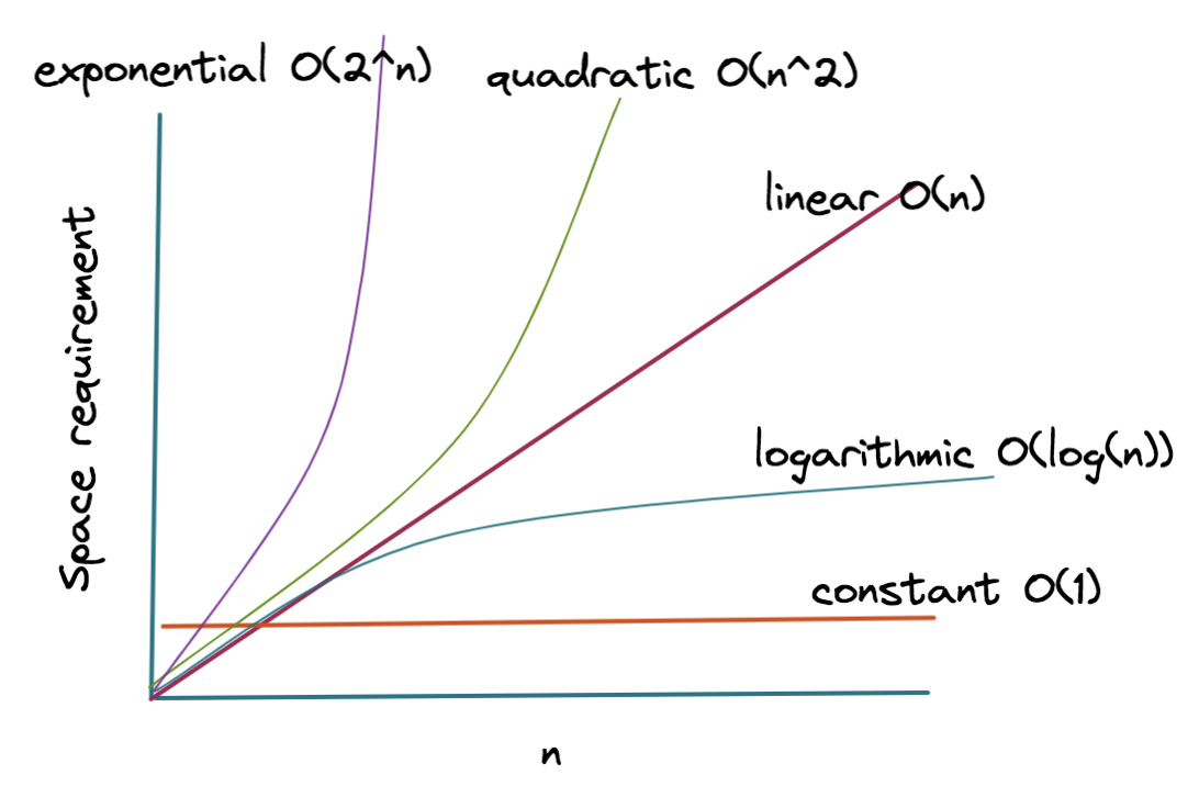
Space complexity describes how the amount of memory an algorithm uses changes with the size of the input. It measures the efficiency of an algorithm in terms of the memory it requires.

Example 1: An Array

Description: Stores n elements in an array.
Space Complexity: O(n)

The amount of memory required grows linearly with the size of the array.

Example 2: A Recursive Function

Description: Calls itself n times before reaching the base case, with each call adding a new frame to the call stack.
Space Complexity: O(n)

The amount of memory required for the call stack grows linearly with the number of recursive calls.

Big O Notation

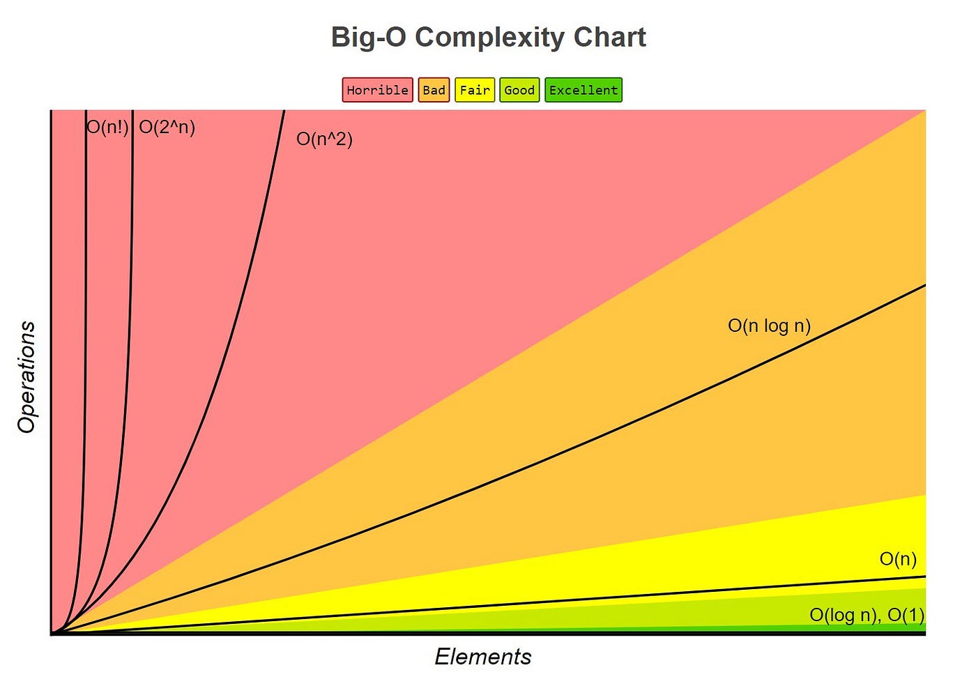
Big O notation describes the upper bound of an algorithm's complexity. Common Big O notations include:

O(1): Constant time/space. Complexity does not change with the size of the input.
O(log n): Logarithmic time/space. Complexity grows logarithmically with the size of the input.
O(n): Linear time/space. Complexity grows linearly with the size of the input.
O(n log n): Linearithmic time/space. Complexity grows faster than linear but slower than quadratic.
O(n^2): Quadratic time/space. Complexity grows quadratically with the size of the input.
O(2^n): Exponential time/space. Complexity grows exponentially with the size of the input.

Summary

Time Complexity: Measures how the runtime of an algorithm changes with the size of the input.
- Examples: Linear search (O(n)), Binary search (O(log n))
Space Complexity: Measures how the memory usage of an algorithm changes with the size of the input.
- Examples: An array of size n (O(n)), A recursive function with n calls (O(n))

Analyzing the time and space complexities of algorithms helps in choosing the most efficient one for handling large inputs.

Pattern Solving

Pattern solving involves identifying and solving repetitive or structured problems. It enhances logical thinking and coding skills.

Examples of Patterns:

Star Patterns
Number Patterns
Alphabet Patterns

C++ STL (Standard Template Library)

The C++ Standard Template Library (STL) provides a set of common classes and interfaces for data structures and algorithms.

Introduction to C++ STL

What is C++ STL?

C++ is one of the most popular high-level programming languages, extensively used by developers for a long time and always loved by all programmers, especially competitive programmers, because of its faster execution time.

STL is one of the unique abilities of C++ which makes it stand out from every other programming language. STL stands for Standard Template Library, which contains a lot of pre-defined templates in terms of containers and classes. This makes it very easy for developers or programmers to implement different data structures easily without having to write complete code and worry about space-time complexities.

If you dive a little deeper into STL, you will have to understand everything about templates and how they work, which is one of the most powerful tools when it comes to the C++ programming language.

However, in this tutorial, we will stick to some of the most popular STL containers and algorithms, and their useful functions, which are used by programmers very frequently in day-to-day programming.

STL Containers and Algorithms

unordered_set in C++ STL
Vector in C++ STL
Set in C++ STL
unordered_multiset in C++ STL
multiset in C++ STL
unordered_map in C++ STL
map in C++ STL
unordered_multimap in C++ STL
queue in C++ STL
stack in C++ STL
deque in C++ STL
priority_queue in C++ STL
multimap in C++ STL
list in C++ STL
next_permutation in STL
__builtin_popcount() in STL
sort() in C++ STL
min_element() in C++ STL
max_element() in C++ STL

Key Components:

Vectors
Stacks
Queues
Deques
Lists
Maps
Sets

Components of STL

STL has four major components:

Containers
Iterators
Algorithms
Function objects

Containers

If you are dealing with many elements, then you need to use some sort of container. Containers can be described as objects that are used to store the collection of data. They help in recreating and implementing complex data structures efficiently.

Containers are further classified into three categories:

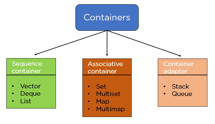
Sequence Containers: These are used to implement sequential data structures like a linked list, array, etc.
Associative Containers: These are containers in which each element has a value that is related to a key. They are used to implement sorted data structures, for example, set, multiset, map, etc.
Container Adapters: Container adapters can be defined as an interface used to provide functionality to the pre-existing containers.

Sequence Container:

Vectors: Vectors can be defined as a dynamic array or an array with some additional features.

Syntax:
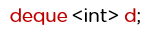
Dequeue: Deque is also known as a double-ended queue that allows inserting and deleting from both ends; they are more efficient than vectors in case of insertion and deletion.

Syntax:
List: List is also the sequential container and allows non-contiguous allocation. It allows insertion and deletion anywhere in the sequence.

Syntax:

Associative Container

Set

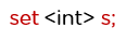
Set is an associative container that is used to store elements that are unique.

Syntax:

Multiset

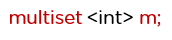
This container is similar to that of the set container; the only difference is that it stores non-unique elements.

Syntax:

Map

Map container contains sets of key-value pairs where each key is associated with one value.

Syntax:

Here, the int is the key type, and the int is the value type.

Multimap

These containers also store key-value pairs, but unlike maps, they can have duplicate elements.

Syntax:

Container Adapter

Stack

Stack follows the last-in, first-out (LIFO) approach, which means new elements are added at the end and removed from that end only.

Queue

Queue follows the first-in, first-out (FIFO) approach, which means new elements are added from the end and removed from the front.

Example:

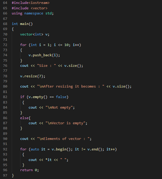
In the above example, you are using vector functions and some other functions to do some operations. After declaring the vector v, you add the elements inside the vector using the push_back() function and with the help of the loop. After that, you are displaying the size of the vector using the size() function. Now using the resize() function, you are resizing the vector size to 7.

Using the empty() function, you check if the vector is empty; if it’s false, then you will display "not empty," and if it is not false, then you will display "the vector is empty."

After that, you display all the vector elements using a for loop and functions like begin() and end(), pointing to the first element and the last element, respectively. Iterators are used to access data in the containers, and they help in traversing through elements of containers using their functions. They can be incremented and decremented as per choice and help in the manipulation of data in the container.

Iterators

Iterators are used to access data in the containers, and it helps in traversing through elements of containers using its functions. They can be incremented and decremented as per choice and help in the manipulation of data in the container.

Iterator Functions

begin(): This function points the iterator to the first element of the container.
end(): This function points the iterator to the position past the last element of the container.

Algorithms

In STL, different types of algorithms can be implemented with the help of iterators. Algorithms can be defined as functions applied to the containers and provide operations for the content of the container. Examples include: sort(), swap(), min(), max(), etc.

Types of Algorithms

Modifying algorithms
Non-modifying algorithms
Sorting algorithms
Searching algorithms
Numeric algorithms

Function Objects

A function object, also known as a functor, is an object of a class that provides a definition for the operator(). Suppose you have declared an object of some class, then you can use that object just like a function.

Conclusion

After reading this tutorial on C++ STL, you should have understood the Standard Template Library and generic programming and all the components of STL in C++, like containers, iterators, and algorithms, in detail. You also learned about function objects along with some examples.

Basic Maths

Basic mathematical concepts are essential for understanding and solving algorithmic problems.

Key Topics:

Prime Numbers
GCD and LCM
Modular Arithmetic
Probability and Combinatorics

Challenges

Count Digits - Easy
- Write a function to count the number of digits in a given number.
Reverse a Number - Easy
- Create a function to reverse the digits of a given number.
Check Palindrome - Easy
- Implement a function to check if a given number or string is a palindrome.
GCD or HCF - Easy
- Write a function to find the Greatest Common Divisor (GCD) or Highest Common Factor (HCF) of two given numbers.
Armstrong Numbers - Easy
- Create a function to check if a given number is an Armstrong number.
Print all Divisors - Easy
- Implement a function to print all divisors of a given number.
Check for Prime - Easy
- Write a function to check if a given number is a prime number.

Introduction to Recursion

Recursion is a method where the solution to a problem depends on solutions to smaller instances of the same problem.

Key Concepts:

Base Case and Recursive Case
Recursive Functions
Stack Memory
Tail Recursion

Recursion is a fundamental concept in computer science and is extensively used in data structures and algorithms. This document provides a comprehensive overview of recursion, its importance, and how it is used in DSA.

What is Recursion?

Recursion is a technique where a function calls itself in order to solve a problem. A problem is divided into smaller instances of the same problem, and each instance is solved using the same algorithm.

How Recursion Works

When a recursive function is called, the following steps are executed:

The current state of the function (variables, execution point) is saved.
The function processes the base case.
If the base case is not met, the function calls itself with a modified argument.
Each call adds a new layer to the call stack until the base case is reached.
Once the base case is reached, the function returns its result, and the stack is unwound.

Base Case and Recursive Case

Base Case

The base case is the condition under which the recursion ends. Without a base case, the function would call itself indefinitely, leading to a stack overflow.

Recursive Case

The recursive case is the part of the function where the function calls itself with a modified argument. This step brings the problem closer to the base case.

Advantages and Disadvantages of Recursion

Advantages

Simplifies the code for complex problems.
Naturally fits problems that can be divided into similar sub-problems.
Useful for tree and graph traversal.

Disadvantages

Can lead to high memory usage due to call stack.
May result in slower execution compared to iterative solutions.
Risk of stack overflow if the base case is not defined properly.

Common Recursive Algorithms

Factorial Calculation: Computes the factorial of a number.
Fibonacci Sequence: Generates numbers in the Fibonacci sequence.
Tree Traversal: Inorder, Preorder, and Postorder traversals of a tree.
Graph Traversal: Depth-First Search (DFS).
Divide and Conquer Algorithms: Quick Sort, Merge Sort.

Recursion vs Iteration

While recursion involves function calls, iteration uses looping constructs like for and while. Recursion is often more intuitive for problems that can be broken down into similar sub-problems, but it can be less efficient in terms of memory and execution time.

Examples

Factorial

def factorial(n):
    if n == 0:
        return 1  # Base case
    else:
        return n * factorial(n - 1)  # Recursive case

      def fibonacci(n):
    if n <= 1:
        return n  # Base case
    else:
        return fibonacci(n - 1) + fibonacci(n - 2)  # Recursive case

int binary_search(int arr[], int low, int high, int x) {
    if (high >= low) {
        int mid = (high + low) / 2;
        if (arr[mid] == x) {
            return mid;
        } else if (arr[mid] > x) {
            return binary_search(arr, low, mid - 1, x);
        } else {
            return binary_search(arr, mid + 1, high, x);
        }
    } else {
        return -1;  // Element is not present in array
    }
}

Recursion

Pre-requisite

The learner must know how to write a basic function in any language and how to make a function call from the main function.

What is Recursion?

It is a phenomenon when a function calls itself indefinitely until a specified condition is fulfilled.

Let's understand recursion with the help of an illustration:

As we can see in the above image, a function is calling the same function inside its body. Since there is no condition to stop the recursive calls, the calls will run indefinitely until the stack runs out of memory (stack overflow).

What is Stack Overflow in Recursion?

Whenever recursion calls are executed, they're simultaneously stored in a recursion stack where they wait for the completion of the recursive function. A recursive function can only be completed if a base condition is fulfilled and the control returns to the parent function.

But, when there is no base condition given for a particular recursive function, it gets called indefinitely which results in a Stack Overflow i.e, exceeding the memory limit of the recursion stack and hence the program terminates giving a Segmentation Fault error.

The illustration above also represents the case of a Stack Overflow as there is no terminating condition for recursion to stop, hence it will also result in a memory limit exceeded error.

Base Condition

It is the condition that is written in a recursive function in order for it to get completed and not to run infinitely. After encountering the base condition, the function terminates and returns back to its parent function simultaneously.

To get a better understanding of how the base condition is an integral part of recursive functions, let us see an example below:

Let's say we have to print integers starting from 0 till 2 only, this will be how the pseudocode for it will look like:

int count = 0;
void func(){
if(count == 3 ) return;
print(count);
count++;
func();
}
main()
{
print();
}

According to this pseudocode, the function will increment and print the value of count and then return when the base condition becomes true i.e, it will only print 0,1,2 and 3 and then execution gets completed.

Recursive code for printing numbers from 0 to 3:

C++

#include<bits/stdc++.h>
using namespace std;
int cnt = 0;

void print(){
   // Base Condition.
   if(cnt == 3)  return;
   cout<<cnt<<endl;

   // Count Incremented
   cnt++;
   print();
}

int main(){
    print();
    return 0;
}

Output

0 1 2

Recursive Tree

A recursive tree is a visual representation of recursion, illustrating how functions are called and returned in a series of consecutive events. It provides a pictorial description of the recursive process.

Key Concepts

Function Calls: The tree shows how functions are called recursively.
Return Flow: It depicts how control returns to parent functions.
Execution Order: The tree illustrates the sequence of function executions.

Process

Functions are called recursively, branching out in the tree structure.
When a recursive call completes, control returns to its parent function.
The parent function continues execution.
This process repeats until the last function in the recursive stack returns.

Importance

Recursive trees help in:

Visualizing the flow of recursive algorithms
Understanding the order of function calls and returns
Analyzing the depth and complexity of recursive processes

Hashing

Hashing is a technique used to uniquely identify a specific object from a group of similar objects.

Key Concepts:

Hash Functions
Collision Handling (Chaining, Open Addressing)
Hash Tables Hashing is a crucial concept in computer science, used extensively for fast data retrieval. This document provides an in-depth look at hashing, its importance in DSA, and examples in C++.

What is Hashing?

Hashing is a technique used to uniquely identify a specific object from a group of similar objects. It is used to map data of arbitrary size to fixed-size values, typically using a hash function. The output, known as a hash value or hash code, is used as an index to store data in a hash table.

Hash Function

A hash function is a function that takes input (or 'key') and returns a fixed-size string of bytes. The output is typically a numerical value which serves as an index to an array. A good hash function should minimize the probability of collisions and distribute keys uniformly across the hash table.

Example:

int hashFunction(int key, int tableSize) {
    return key % tableSize;
}

Hash Table

A hash table is a data structure that implements an associative array, a structure that can map keys to values. Hash tables use a hash function to compute an index into an array of buckets or slots, from which the desired value can be found.

Collision Handling

Collisions occur when two keys hash to the same index. Several methods exist to handle collisions:

Separate Chaining

Separate chaining involves maintaining a list of all elements that hash to the same value. This is typically implemented using linked lists.

Open Addressing

Open addressing stores all elements in the hash table itself. When a collision occurs, the algorithm searches for the next available slot using a probing sequence.

Advantages and Disadvantages of Hashing

Advantages

Fast data retrieval
Efficient memory usage
Simple implementation

Disadvantages

Collisions can degrade performance
Hash functions can be complex to design
Inefficient for small datasets

Common Applications of Hashing

Implementing associative arrays
Database indexing
Caching
Password storage
Data de-duplication

Best Practices

Choose a good hash function: Ensure it distributes keys uniformly.
Handle collisions efficiently: Select the appropriate method based on the use case.
Consider table size: Avoid too many collisions by choosing an appropriate size.
Rehashing: Dynamically resize the hash table when it becomes too full.

By understanding and applying these principles, you can effectively use hashing to solve a variety of problems in data structures and algorithms.

Sorting

Sorting is the process of arranging data in a particular order. It is a fundamental operation in computer science.

Common Sorting Algorithms:

Bubble Sort
Selection Sort
Insertion Sort
Merge Sort
Quick Sort
Heap Sort
Sorting Algorithms in C++

Sorting is a fundamental operation in computer science that arranges elements of a list in a particular order. This document covers various sorting algorithms and their implementations in C++.

Selection Sort

Selection Sort is a simple sorting algorithm that repeatedly selects the minimum (or maximum) element from the unsorted portion and swaps it with the first unsorted element.

Implementation in C++

void selectionSort(int arr[], int n) {
    for (int i = 0; i < n - 1; ++i) {
        int min_index = i;
        for (int j = i + 1; j < n; ++j) {
            if (arr[j] < arr[min_index]) {
                min_index = j;
            }
        }
        swap(arr[i], arr[min_index]);
    }
}

      void bubbleSort(int arr[], int n) {
    for (int i = 0; i < n - 1; ++i) {
        bool swapped = false;
        for (int j = 0; j < n - i - 1; ++j) {
            if (arr[j] > arr[j + 1]) {
                swap(arr[j], arr[j + 1]);
                swapped = true;
            }
        }
        if (!swapped) break;
    }
}

  
cpp
void insertionSort(int arr[], int n) {
    for (int i = 1; i < n; ++i) {
        int key = arr[i];
        int j = i - 1;
        while (j >= 0 && arr[j] > key) {
            arr[j + 1] = arr[j];
            --j;
        }
        arr[j + 1] = key;
    }
}

Best Practices for Sorting Algorithms

Sorting algorithms are essential tools in computer science for arranging data in a particular order. To effectively utilize sorting algorithms, consider the following best practices:

Choose the appropriate algorithm: Different sorting algorithms have different performance characteristics (e.g., time complexity, space complexity). Select an algorithm based on the size of the data set and its nature (e.g., already partially sorted, uniformly distributed).
Understand the algorithm's complexity: Familiarize yourself with the time and space complexity of each sorting algorithm. This knowledge helps in making informed decisions about which algorithm to use based on the expected size of the data and available memory.
Test with various input sizes: Validate the sorting algorithm's performance with different input sizes. Test with small, medium, and large datasets to ensure it performs efficiently across various scenarios and doesn't exhibit unexpected behavior for specific inputs.
Consider stability: Some sorting algorithms are stable, meaning they maintain the relative order of equal elements (elements with the same key). If preserving the original order of equal elements is important in your application, choose a stable sorting algorithm.

By adhering to these best practices and understanding the principles behind sorting algorithms, you can effectively choose and implement sorting solutions that meet the requirements of different applications and datasets.

Bit Manipulation

Bit manipulation is an essential topic in computer science and programming. It involves manipulating bits, the smallest unit of data in a computer. This README provides a comprehensive guide on various aspects of bit manipulation including binary number conversions, 1's and 2's complements, and bitwise operators.

Binary Number Conversions

Binary number conversions are fundamental in understanding bit manipulation. Here, we explore various conversions involving binary numbers.

Decimal to Binary

To convert a decimal number to binary, divide the number by 2 and record the remainder. Repeat this process with the quotient until the quotient is zero. The binary representation is the sequence of remainders read in reverse order.

Example:

Decimal: 10
Binary: 1010

Binary to Decimal

To convert a binary number to decimal, multiply each bit by 2 raised to the power of its position from the right (starting from 0) and sum the results.

Example:

Binary: 1010
Decimal: (1 \times 2^3 + 0 \times 2^2 + 1 \times 2^1 + 0 \times 2^0 = 8 + 0 + 2 + 0 = 10)

Binary to Hexadecimal

To convert binary to hexadecimal, group the binary digits into sets of four (starting from the right) and convert each set to its hexadecimal equivalent.

Example:

Binary: 10101100
Grouped: 1010 1100
Hexadecimal: AC

Hexadecimal to Binary

To convert hexadecimal to binary, convert each hexadecimal digit to its 4-bit binary equivalent.

Example:

Hexadecimal: AC
Binary: 1010 1100

Binary to Octal

To convert binary to octal, group the binary digits into sets of three (starting from the right) and convert each set to its octal equivalent.

Example:

Binary: 10101100
Grouped: 010 101 100
Octal: 254

Octal to Binary

To convert octal to binary, convert each octal digit to its 3-bit binary equivalent.

Example:

Octal: 254
Binary: 010 101 100

1's and 2's Complements

1's and 2's complements are methods to represent negative numbers in binary.

1's Complement

1's complement of a binary number is obtained by inverting all bits (changing 1s to 0s and 0s to 1s).

Example:

Binary: 1010
1's Complement: 0101

2's Complement

2's complement is obtained by adding 1 to the 1's complement of the number. It is widely used in computer systems to represent negative numbers.

Example:

Binary: 1010
1's Complement: 0101
2's Complement: 0101 + 1 = 0110

Bitwise Operators

Bitwise operators are used to perform operations on individual bits of binary numbers. Here we discuss common bitwise operators.

AND Operator

The AND operator (&) performs a logical AND operation on each pair of corresponding bits of two numbers. The result is 1 only if both bits are 1.

Example:

1010
AND 0110
Result: 0010

OR Operator

The OR operator (|) performs a logical OR operation on each pair of corresponding bits of two numbers. The result is 1 if at least one of the bits is 1.

Example:

1010
OR 0110
Result: 1110

XOR Operator

The XOR operator (^) performs a logical XOR operation on each pair of corresponding bits of two numbers. The result is 1 if only one of the bits is 1.

Example:

1010
XOR 0110
Result: 1100

NOT Operator

The NOT operator (~) inverts all bits of a number (changing 1s to 0s and 0s to 1s).

Example:

Binary: 1010
NOT: 0101

Shift Operators

Shift operators shift the bits of a number to the left or right. They include left shift (<<) and right shift (>>).

Left Shift (<<)

The left shift operator shifts bits to the left by a specified number of positions. Bits shifted out from the left are discarded, and zero bits are shifted in from the right.

Example:

Binary: 1010
Left Shift by 2: 101000

Right Shift (>>)

The right shift operator shifts bits to the right by a specified number of positions. Bits shifted out from the right are discarded, and zero bits are shifted in from the left.

Example:

Binary: 1010
Right Shift by 2: 0010

Bitwise operations are fundamental in low-level programming and are extensively used in system programming, cryptography, network programming, and more. Understanding these concepts is crucial for efficient coding and optimization.

Dynamic Programming

Dynamic programming is a method for solving complex optimization problems by breaking them down into simpler subproblems, solving each of these subproblems just once, and storing their solutions. The stored solutions are then reused whenever needed, thus reducing the computation time significantly.

This approach is particularly useful for problems with overlapping subproblems and optimal substructure properties. Dynamic programming is widely used across different domains, from algorithm design to various real-world applications.

Introduction

Dynamic programming (DP) is a mathematical optimization method and a computer programming approach. Unlike divide and conquer algorithms, which solve subproblems independently, dynamic programming solves each subproblem only once and stores its result for future use.

The term "dynamic programming" was coined by Richard Bellman in the 1950s. He used it to solve multi-stage decision processes where decisions at one stage affect subsequent stages. This approach has become a cornerstone in both algorithm design and operational research.

Why Use Dynamic Programming?

Efficiency: It reduces the time complexity of algorithms from exponential to polynomial time by storing solutions of subproblems.
Reusability: Once a subproblem is solved, its solution can be reused multiple times, making the process efficient.
Optimal Solutions: Dynamic programming ensures finding the most efficient solution to a problem by systematically exploring all possible solutions.

Dynamic programming is especially useful for problems with a large number of overlapping subproblems and problems where finding the optimal solution involves combining solutions of subproblems in a recursive manner.

Key Concepts

Dynamic programming is based on two key principles:

Overlapping Subproblems

Overlapping subproblems arise when a recursive algorithm revisits the same problem multiple times. This is typical in problems that can be solved using recursion where a function calls itself with the same arguments repeatedly.

Example Explanation: Consider a problem of computing Fibonacci numbers. The naive recursive approach recalculates the same Fibonacci numbers multiple times, leading to redundant calculations. Instead, by storing already computed Fibonacci numbers, dynamic programming solves this problem efficiently.

Identifying Overlapping Subproblems: A problem is said to have overlapping subproblems if it can be broken down into subproblems which are reused multiple times. This characteristic is crucial for applying dynamic programming.
Efficiency Gain: By solving each subproblem only once and storing the results, dynamic programming avoids the redundant computation, thereby enhancing efficiency significantly.

Common Problems with Overlapping Subproblems:

Fibonacci Sequence
Longest Common Subsequence
Edit Distance

Optimal Substructure

Optimal substructure means that an optimal solution to the problem contains optimal solutions to the subproblems. This property allows a problem to be solved using dynamic programming.

Example Explanation: In the shortest path problem, the optimal path from a starting node to an ending node is composed of optimal paths between intermediate nodes. Thus, solving subproblems optimally helps in solving the larger problem optimally.

Identifying Optimal Substructure: If a problem can be solved by breaking it down into smaller subproblems, and the solutions to these subproblems can be combined to form a solution to the original problem, it exhibits optimal substructure.
Importance: This property is critical for applying dynamic programming techniques, as it ensures that solving subproblems optimally guarantees an optimal solution to the overall problem.

Common Problems with Optimal Substructure:

Knapsack Problem
Matrix Chain Multiplication
Travelling Salesman Problem

Approaches to Dynamic Programming

Dynamic programming can be implemented using two main approaches, each with its own characteristics and use cases.

Top-Down Approach (Memoization)

The top-down approach, also known as memoization, involves solving problems recursively and storing the results of already solved subproblems to avoid recalculations.

How It Works: Start with the original problem and recursively break it down into subproblems. Store the solutions to subproblems in a data structure, usually a map or array, so that when the same subproblem is encountered again, the stored result can be used.
Characteristics:
- Recursive function calls.
- Uses additional data structures (like arrays or hash tables) for storage.
- Can be easier to implement for problems with a natural recursive structure.
Advantages:
- Simplicity: Easier to write and understand if the problem has a recursive structure.
- Reusability: Efficiently uses recursion with stored results to avoid redundant calculations.
Disadvantages:
- Space Overhead: Requires additional space to store solutions to subproblems.
- Stack Overflow: Recursive calls may lead to stack overflow for problems with large input sizes.
Use Cases: Top-down approaches are often used in problems where the natural structure of the problem leads to recursive solutions, such as Fibonacci numbers or certain graph problems.

Example Explanation: In computing the nth Fibonacci number using memoization, instead of recalculating previously computed Fibonacci numbers, they are stored in an array or dictionary for future reference. This eliminates redundant computations and reduces the overall time complexity.

Bottom-Up Approach (Tabulation)

The bottom-up approach, or tabulation, solves problems iteratively by building up solutions from the simplest subproblems to the desired complex solution.

How It Works: Start by solving the smallest subproblems and use these solutions to iteratively solve larger subproblems, eventually solving the original problem.
Characteristics:
- Iterative approach using loops.
- Utilizes tables or arrays to store solutions of subproblems.
- Constructs solutions systematically from base cases up to the original problem.
Advantages:
- Space Efficiency: Typically requires less memory than memoization since it doesn’t rely on the call stack.
- No Stack Overflow: Avoids the risk of stack overflow as it doesn't involve deep recursive calls.
Disadvantages:
- Complexity: May be harder to implement for problems where the recursive structure is more apparent.
- Initialization: Requires careful initialization of the table and iteration order.
Use Cases: Bottom-up approaches are preferred when the problem can be broken down into a set of subproblems that can be solved iteratively, such as in problems involving sequences or arrays like the longest common subsequence.

Example Explanation: In finding the longest common subsequence between two strings, the bottom-up approach builds a table that iteratively calculates the length of the subsequence for increasing substrings of the input strings. This allows for a systematic exploration of all possibilities, storing intermediate results in a table for later use.

Comparison: Top-Down vs Bottom-Up

Feature	Top-Down (Memoization)	Bottom-Up (Tabulation)
Approach	Recursive	Iterative
Space Usage	Higher (due to recursion)	Lower (usually)
Ease of Use	Simple for recursive problems	Complex problems with no natural recursion
Stack Risk	Possible stack overflow	No risk of stack overflow
Performance	Often similar, depends on problem	Often similar, depends on problem

Applications of Dynamic Programming

Dynamic programming is a versatile and powerful tool applied across numerous domains. Here are some of its most well-known applications:

1. Fibonacci Sequence Calculation

Description: Calculate Fibonacci numbers, where each number is the sum of the two preceding ones.

Application: In mathematical computations, analysis of algorithms, and many other scientific applications.
Dynamic Programming Use: Store previously calculated Fibonacci numbers to avoid recalculating them, reducing time complexity from exponential to linear.

2. Knapsack Problem

Description: Determine the maximum value that can be achieved with a given weight capacity of a knapsack and a set of items with given weights and values.

Application: Resource allocation, financial decision-making, and other optimization scenarios.
Dynamic Programming Use: Solve subproblems of smaller capacity knapsacks, storing results to build up to the desired capacity, thereby ensuring optimal resource utilization.

3. Longest Common Subsequence (LCS)

Description: Find the longest subsequence common to two sequences, which may not necessarily be contiguous.

Application: Bioinformatics for DNA sequence alignment, text processing, and version control systems.
Dynamic Programming Use: Build a matrix to compare all subsequences and store intermediate results, allowing efficient identification of the longest common subsequence.

4. Edit Distance Problem

Description: Calculate the minimum number of edits (insertions, deletions, substitutions) required to convert one string into another.

Application: Spell checkers, natural language processing, and genetic sequence alignment.
Dynamic Programming Use: Use a matrix to represent the transformation costs between all possible prefixes of the two strings, iteratively filling the matrix to determine the minimum edit distance.

5. Optimal Binary Search Tree (OBST)

Description: Construct a binary search tree with minimal expected search cost based on a set of keys with given access probabilities.

Application: Database indexing, search algorithms, and data retrieval systems.
Dynamic Programming Use: Solve subproblems for smaller trees and combine solutions to determine the optimal cost for larger trees, ensuring minimal access cost.

6. Matrix Chain Multiplication

Description: Find the most efficient way to multiply a given sequence of matrices.

Application: Computer graphics, scientific computing, and performance optimization.
Dynamic Programming Use: Determine the cost of multiplying every possible combination of matrices, storing results in a table to minimize overall computation cost.

7. Travelling Salesman Problem (TSP)

Description: Find the shortest possible route that visits each city exactly once and returns to the origin city.

Application: Route optimization, logistics, and transportation planning.
Dynamic Programming Use: Solve subproblems for paths through subsets of cities and use these to build up to the complete route, ensuring the shortest path is found.

8. Rod Cutting Problem

Description: Given a rod of length n and a set of prices for each length, determine the maximum revenue obtainable by cutting up the rod and selling the pieces.

Application: Resource optimization in manufacturing, financial modeling, and supply chain management.
Dynamic Programming Use: Solve subproblems for different lengths and store results to maximize revenue for the full rod.

9. Coin Change Problem

Description: Determine the minimum number of coins needed to make a specific amount using given coin denominations.

Application: Financial calculations, vending machines, and cash register systems.
Dynamic Programming Use: Build a table of solutions for smaller amounts, iteratively calculating the minimum number of coins needed for larger amounts.

10. Subset Sum Problem

Description: Determine if there is a subset of a given set of integers that adds up to a specific target sum.

Application: Cryptography, partitioning problems, and combinatorial optimization.
Dynamic Programming Use: Solve subproblems for smaller subsets and store results to efficiently determine if the target sum is achievable.

Real-World Applications

Bioinformatics: Dynamic programming is extensively used in bioinformatics for DNA sequence alignment and protein structure prediction, enabling the efficient comparison and analysis of genetic data.
Speech Recognition: Algorithms like the Hidden Markov Model (HMM) utilize dynamic programming for efficient computation of speech patterns and recognition of spoken words.
Finance: In finance, dynamic programming helps solve complex decision-making problems like portfolio optimization and risk management by efficiently exploring all possible investment strategies.
Operations Research: Dynamic programming is used in operations research for solving multi-stage decision problems, such as supply chain optimization and resource allocation, to achieve optimal outcomes.
Game Theory: Dynamic programming techniques are applied in game theory to analyze and solve complex strategic interactions between players, determining optimal strategies and outcomes.

Advantages and Limitations

Advantages

Efficiency: Dynamic programming reduces time complexity by storing and reusing solutions to subproblems, avoiding redundant computations and significantly speeding up algorithms.
Reusability: Once a subproblem is solved, its solution can be reused multiple times, enhancing efficiency and performance in solving larger problems.
Optimal Solutions: Dynamic programming ensures finding the most efficient solution to a problem by systematically exploring all possible solutions and selecting the best one.
Versatility: Applicable to a wide range of problems across different domains, from computer science to operations research, finance, and more.
Deterministic: Provides deterministic solutions that guarantee optimal results for problems with overlapping subproblems and optimal substructure.

Limitations

Space Complexity: Storing solutions to subproblems can lead to high space complexity, especially for problems with a large number of subproblems or large input sizes.
Complexity: Designing dynamic programming solutions requires a deep understanding of the problem's structure and can be more complex compared to other techniques.
Not Always Suitable: Dynamic programming is not suitable for problems that do not exhibit optimal substructure or overlapping subproblems, limiting its applicability.
Initialization Overhead: Careful initialization of tables or data structures is required, which can add complexity to the implementation.
Problem-Specific: Dynamic programming solutions are often highly problem-specific and may not generalize well to other problems.

Conclusion

Dynamic programming is a powerful and efficient method for solving complex optimization problems that exhibit overlapping subproblems and optimal substructure properties. By breaking problems down into simpler subproblems, storing their solutions, and reusing these solutions, dynamic programming significantly reduces computation time and ensures optimal solutions.

This technique is widely used across various domains, from algorithm design to real-world applications like bioinformatics, finance, and operations research. Understanding and applying dynamic programming concepts can greatly enhance problem-solving skills and improve the efficiency of algorithms.

Linked List

Definition

A Linked List is a linear data structure where elements are stored in nodes. Each node contains a data part and a reference (or pointer) to the next node in the sequence.

Types:

Singly Linked List: Each node points to the next node.
Doubly Linked List: Each node points to both the next and the previous nodes.
Circular Linked List: The last node points back to the first node.

Operations:

Insertion: Add elements at the beginning, end, or at a specific position.
Deletion: Remove elements from the beginning, end, or a specific position.
Traversal: Go through each node starting from the head.

Time Complexity:

Insertion: O(1) at the head, O(n) for arbitrary position.
Deletion: O(1) for head, O(n) for arbitrary position.
Search: O(n)

Stack

Definition

A Stack is a linear data structure that follows the LIFO (Last In, First Out) principle. The last element added is the first one to be removed.

Operations:

Push: Add an element to the top.
Pop: Remove the top element.
Peek/Top: Return the top element without removing it.
IsEmpty: Check if the stack is empty.

Applications:

Function call management (recursion).
Undo operations in text editors.
Expression evaluation and syntax parsing.

Time Complexity:

Push, Pop, Peek: O(1)

Queue

Definition

A Queue is a linear data structure that follows the FIFO (First In, First Out) principle. The first element added is the first one to be removed.

Types:

Simple Queue: Basic FIFO structure.
Circular Queue: The last element points back to the first.
Priority Queue: Elements are dequeued based on priority rather than insertion order.

Operations:

Enqueue: Add an element to the rear.
Dequeue: Remove the front element.
Front: Get the front element without removing it.
IsEmpty: Check if the queue is empty.

Applications:

CPU scheduling.
Printer queue management.
BFS (Breadth-First Search) in graphs.

Time Complexity:

Enqueue, Dequeue: O(1)

Trees

Definition

A Tree is a hierarchical data structure with a root node and children represented as a set of linked nodes. It has a recursive structure, meaning each subtree is also a tree.

Types:

Binary Tree: Each node has at most two children.
Binary Search Tree (BST): A binary tree where the left child node contains values smaller than the parent and the right child node contains values greater than the parent.
AVL Tree: A self-balancing binary search tree.
Heap: A complete binary tree used in heap sort.

Operations:

Insertion: Insert nodes at appropriate positions.
Deletion: Remove a node and rearrange the tree.
Traversal: In-order, Pre-order, Post-order, Level-order.

Applications:

Hierarchical data representation (e.g., file systems).
Expression parsing in compilers.
Database indexing (B-Trees).

Time Complexity:

Search, Insertion, Deletion: O(log n) for balanced trees, O(n) for unbalanced trees.

Graphs

Definition

A Graph is a collection of nodes (called vertices) and edges connecting them. Graphs can be directed or undirected.

Types:

Undirected Graph: Edges have no direction.
Directed Graph (Digraph): Edges have a direction.
Weighted Graph: Edges have weights.

Representation:

Adjacency Matrix: A 2D array to represent connections.
Adjacency List: A list of lists to represent connections.

Operations:

BFS (Breadth-First Search): Explore neighbors level by level.
DFS (Depth-First Search): Explore as far as possible along a branch.
Shortest Path Algorithms: Dijkstra's, Bellman-Ford.
Minimum Spanning Tree: Prim's, Kruskal's.

Applications:

Social networks, GPS systems, network routing.
Pathfinding in games.

Time Complexity:

BFS, DFS: O(V + E) where V is the number of vertices and E is the number of edges.

Tries

Definition

A Trie (also called a prefix tree) is a specialized tree used to store associative data structures. It is used primarily for quick retrieval of keys, such as words in a dictionary.

Operations:

Insert: Add a word or string to the trie.
Search: Check if a word or string is in the trie.
Prefix Search: Find all strings that start with a given prefix.

Applications:

Autocomplete features.
Spell-checking.
IP routing.

Time Complexity:

Insert, Search: O(L), where L is the length of the word being inserted or searched.

Conclusion

Understanding these fundamental data structures is essential for developing efficient algorithms and solving complex problems in software engineering. Each data structure has its specific use cases, and selecting the right one can significantly optimize the performance of your application.

Name		Name	Last commit message	Last commit date
Latest commit History 133 Commits
Array		Array
Binary Bootcamp		Binary Bootcamp
Bit-Manipulation		Bit-Manipulation
DP		DP
Greedy Algo		Greedy Algo
Hashing		Hashing
Leetcode-75		Leetcode-75
Recursion		Recursion
Revision		Revision
Sorting		Sorting
Strings		Strings
Two Pointer		Two Pointer
Z-basics		Z-basics
.gitignore		.gitignore
README.md		README.md

Folders and files

Latest commit

History

Repository files navigation

Data Structures and Algorithms Learning Guide

Table of Contents

Basics of C++

Time and Space Complexity

Time Complexity

Example 1: Linear Search

Example 2: Binary Search

Space Complexity

Example 1: An Array

Example 2: A Recursive Function

Big O Notation

Summary

Pattern Solving

Examples of Patterns:

C++ STL (Standard Template Library)

Introduction to C++ STL

What is C++ STL?

STL Containers and Algorithms

Key Components:

Components of STL

Containers

Associative Container

Set

Multiset

Map

Multimap

Container Adapter

Stack

Queue

Iterators

Iterator Functions

Algorithms

Types of Algorithms

Function Objects

Conclusion

Basic Maths

Key Topics:

Challenges

Introduction to Recursion

Key Concepts:

Table of Contents

What is Recursion?

How Recursion Works

Base Case and Recursive Case

Base Case

Recursive Case

Advantages and Disadvantages of Recursion

Advantages

Disadvantages

Common Recursive Algorithms

Recursion vs Iteration

Examples

Factorial

Recursion

Pre-requisite

What is Recursion?

What is Stack Overflow in Recursion?

Base Condition

Recursive code for printing numbers from 0 to 3:

C++

Output

Recursive Tree

Key Concepts

Process

Importance

Hashing

Key Concepts:

Table of Contents

What is Hashing?

Hash Function

Example:

Hash Table

Collision Handling

Separate Chaining

Open Addressing

Advantages and Disadvantages of Hashing