⚡ A high-performance PyTorch library for generative modeling
Composable primitives for EBMs, diffusion, flow matching, and Schrödinger bridges.

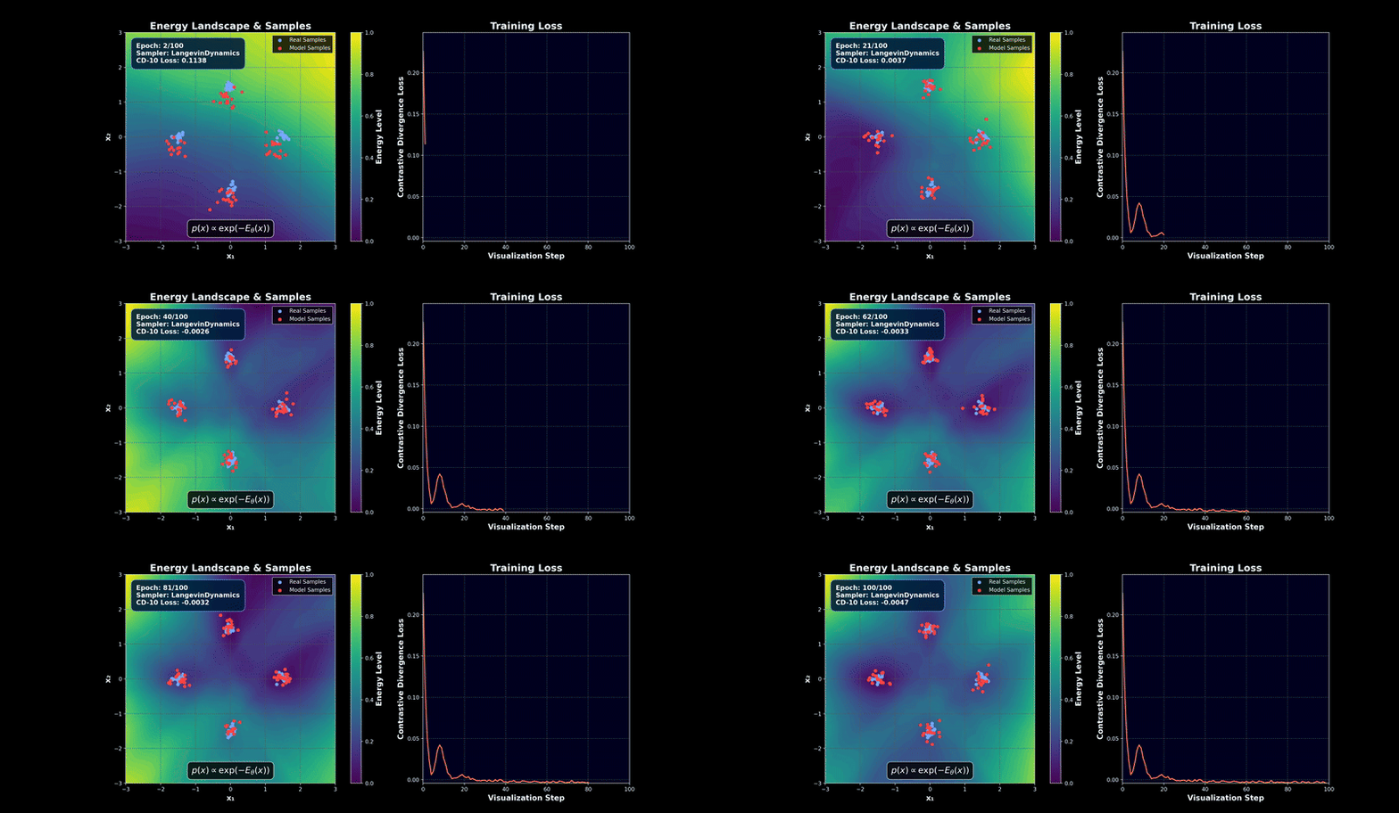
An energy landscape learning to place its low-energy basins on the data.

What is ∇ TorchEBM 🍓?

TorchEBM takes the statistical-mechanics view of generative modeling. A system is described by a scalar potential $E_\theta(x)$, which induces a Boltzmann measure

$$p_\theta(x) ;\propto; e^{-E_\theta(x)/\varepsilon},$$

and generation is the act of relaxing a distribution toward that equilibrium, or of transporting one density onto another along a prescribed path. MCMC is relaxation toward equilibrium, diffusion and flow matching are prescribed transport between densities, and the recent hybrids parameterize the transport by the potential itself.

So TorchEBM implements the components once and lets the method be a configuration:

Component	The question it answers	Package
Energy / field	what is the system?	torchebm.core, torchebm.models
Interpolant	along which path do noise and data connect?	torchebm.interpolants
Coupling	which noise sample is paired with which datum?	torchebm.couplings
Objective	how is the model fit to data?	torchebm.losses
Sampler	which dynamics produce samples?	torchebm.samplers
Integrator	how are those dynamics discretized?	torchebm.integrators

Compose them one way and you have flow matching with optimal-transport couplings; another way and you have contrastive divergence with Langevin negatives; another and you have equilibrium matching, sampled as an ODE or descended as an energy. The Design and Scope page places every method family in this taxonomy, with references.

📚 Full documentation: the TorchEBM website · ⚡ Benchmarks dashboard

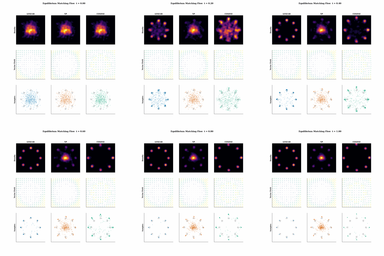
Equilibrium matching: a time-invariant field trained on eight gaussians, then integrated from noise with FlowSampler.

What's inside

Training objectives (torchebm.losses)

Sampling-based objectives buy a calibrated energy at the cost of MCMC in the loop; transport-based objectives replace that inner loop with regression along a path.

Objective	Idea	Inner sampling
ContrastiveDivergence	push energy down on data, up on short-run MCMC negatives; persistent=True gives persistent CD with a replay buffer	yes
ScoreMatching	match the model score to the data score	no
DenoisingScoreMatching	match the score of noise-perturbed data	no
SlicedScoreMatching	estimate the Hessian trace by random projections	no
EquilibriumMatchingLoss	learn a time-invariant equilibrium field; generate as an ODE or descend it as an energy	no
EnergyMatchingLoss	one time-independent potential: optimal-transport flow warm-up, then contrastive sharpening of its Boltzmann density	phase two only

Samplers (torchebm.samplers)

Sampler	Dynamics
LangevinDynamics	overdamped Langevin: gradient descent on the energy plus noise
HamiltonianMonteCarlo	Hamiltonian trajectories with a symplectic integrator and a Metropolis test
RiemannianManifoldHMC	HMC on a position-dependent metric, for ill-conditioned geometry
GradientDescentSampler	noise-free mode seeking
NesterovSampler	momentum-accelerated mode seeking
FlowSampler	continuous-time generation: mode="ode" (probability flow) or mode="sde" (diffusion), from velocity, score, or noise predictions

Numerical integrators (torchebm.integrators)

Every sampler takes integrator= as a registry name or an instance, so the numerics are swappable without touching the model.

Family	Integrators
Explicit Runge-Kutta	HeunIntegrator, Bosh3Integrator, RK4Integrator, RK438Integrator
Adaptive step size	AdaptiveHeunIntegrator, Dopri5Integrator, Dopri8Integrator
Stochastic (SDE)	EulerMaruyamaIntegrator, BackwardEulerMaruyamaIntegrator (implicit)
Symplectic (Hamiltonian)	LeapfrogIntegrator, GeneralisedLeapfrogIntegrator (non-separable)

Paths and pairings (torchebm.interpolants, torchebm.couplings)

The path decides how noise becomes data; the coupling decides which noise becomes which datum. Straighter pairings mean straighter paths and fewer sampling steps.

Interpolants	Couplings
LinearInterpolant (flow matching)	IndependentCoupling (the classical pairing)
CosineInterpolant	GreedyCoupling (nearest unmatched)
VariancePreservingInterpolant (diffusion)	SinkhornCoupling (entropic OT), ExactOTCoupling
	UnbalancedSinkhornCoupling (per-pair weights), ReflowCoupling (model-induced)

And the rest

Energies (GaussianModel, DoubleWellModel, HarmonicModel, RastriginModel, AckleyModel, RosenbrockModel) with known statistics, so sampler behavior is measurable. Architectures (ConditionalTransformer2D, LabelClassifierFreeGuidance, InteractionModel) for image-scale energies and fields. Schedulers (CosineScheduler, WarmupScheduler, TemperatureScheduler, ...) for any parameter that should anneal. Datasets: eight synthetic 2D benchmarks. CUDA acceleration and mixed precision throughout.

Install

pip install torchebm

Usage

Each block below is one method, as published, in as few lines as it takes. Every snippet runs as-is. Annotated, full-scale versions of all of them live in the examples gallery, which is executed in CI.

Sampling an energy

Langevin dynamics: descend the energy, add noise, repeat. Chains are a batch dimension, so 10,000 of them cost one integer.

import torch
from torchebm.core import GaussianModel
from torchebm.samplers import LangevinDynamics

model = GaussianModel(mean=torch.zeros(2), cov=torch.tensor([[1., .8], [.8, 1.]]))
sampler = LangevinDynamics(model=model, step_size=0.02, noise_scale=1.0)

samples = sampler.sample(dim=2, n_samples=10_000, n_steps=500)  # (10000, 2)

Hamiltonian Monte Carlo

MCMC using Hamiltonian dynamics, Neal 2011. Momentum plus a symplectic integrator buys long, decorrelated proposals.

from torchebm.samplers import HamiltonianMonteCarlo

hmc = HamiltonianMonteCarlo(model=model, step_size=0.1, n_leapfrog_steps=10)

samples, diagnostics = hmc.sample(dim=2, n_samples=1000, n_steps=500,
                                  return_diagnostics=True)
diagnostics["acceptance_rate"].mean()   # scalar

Riemannian manifold HMC

Riemann manifold Langevin and Hamiltonian Monte Carlo, Girolami & Calderhead 2011. A position-dependent metric makes the geometry local; the non-separable Hamiltonian is solved by an implicit generalised leapfrog.

from torchebm.samplers import RiemannianManifoldHMC

def metric_fn(x):                                   # (b, d) -> (b, d, d), SPD
    scale = 1.0 + x.pow(2).sum(-1)[:, None, None]
    return torch.eye(2).expand(x.shape[0], 2, 2) * scale

rmhmc = RiemannianManifoldHMC(model=model, metric_fn=metric_fn,
                              step_size=0.05, n_leapfrog_steps=5)
samples = rmhmc.sample(dim=2, n_samples=1000, n_steps=200)

Equilibrium matching

Equilibrium Matching: Generative Modeling with Implicit Energy-Based Models, Wang & Du 2025. Drop time conditioning: learn one equilibrium gradient field instead of a family of time-varying ones, then sample by integrating it or by simply descending it.

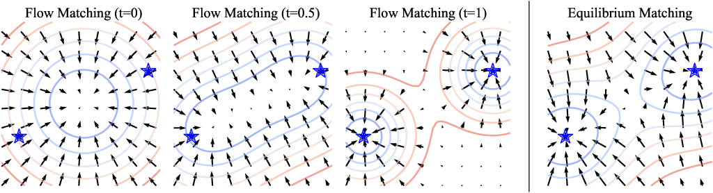
Fig. 1 of Wang & Du (2025): flow matching needs a different field at every $t$ (left); EqM learns one time-invariant field whose minima are the data (right), so sampling becomes optimization.

import torch
from torchebm.core import BaseModel
from torchebm.datasets import TwoMoonsDataset
from torchebm.losses import EquilibriumMatchingLoss
from torchebm.samplers import FlowSampler, NesterovSampler

data = TwoMoonsDataset(n_samples=3000, noise=0.05).get_data()
loss_fn = EquilibriumMatchingLoss(model=field, interpolant="linear", energy_type="dot")
opt = torch.optim.Adam(field.parameters(), lr=1e-3)

for _ in range(3000):
    loss = loss_fn(data[torch.randint(len(data), (256,))])
    opt.zero_grad(); loss.backward(); opt.step()

# generate by integrating the field ...
flow = FlowSampler(model=field, interpolant="linear",
                   negate_velocity=True, integrator="euler")
samples = flow.sample(x=torch.randn(1000, 2), n_steps=100)       # (1000, 2)

# ... or by descending it, because the field is the gradient of an energy
class LearnedEnergy(BaseModel):
    def __init__(self, net):
        super().__init__()
        self.net = net
    def forward(self, x):
        return (x * self.net(x, torch.zeros(x.shape[0]))).sum(-1)

modes = NesterovSampler(LearnedEnergy(field), step_size=0.01,
                        momentum=0.9).sample(n_samples=1000, dim=2, n_steps=200)

Energy matching

Energy Matching: Unifying Flow Matching and Energy-Based Models, Balcerak et al. 2025. One time-independent potential does both jobs: an optimal-transport flow warm-up shapes it far from the data, then a contrastive phase sharpens its Boltzmann density near the data. Generation is a single temperature-scheduled Langevin sweep.

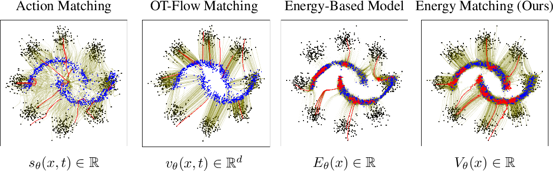
Fig. 1 of Balcerak et al. (2025): a time-independent potential $V_\theta(x)$ (right) both transports and equilibrates, where flow matching needs $v_\theta(x, t)$ and a plain EBM needs long MCMC. Reproduced in the examples.

from torchebm.core import TemperatureScheduler
from torchebm.couplings import SinkhornCoupling
from torchebm.losses import EnergyMatchingLoss
from torchebm.samplers import LangevinDynamics

loss_fn = EnergyMatchingLoss(model=potential, coupling=SinkhornCoupling(reg=0.01),
                             lambda_cd=0.0,          # phase 1: pure OT flow matching
                             epsilon_max=0.15, tau_star=0.8)

for step in range(22_000):
    if step == 20_000:
        loss_fn.lambda_cd = 2.0                      # phase 2: contrastive sharpening
    loss = loss_fn(data[torch.randint(len(data), (128,))])
    opt.zero_grad(); loss.backward(); opt.step()

temperature = TemperatureScheduler(epsilon_max=0.15, tau_star=0.8, n_steps=200, t_end=1.0)
samples = LangevinDynamics(model=potential, step_size=0.01,
                           noise_scale=temperature).sample(x=torch.randn(4000, 2), n_steps=200)

Flow matching

Flow Matching for Generative Modeling, Lipman et al. 2023. Regress a velocity field onto the conditional velocity of a probability path. With TorchEBM's primitives, that is the loop itself.

Fig. 2 of Lipman et al. (2023): the diffusion path's conditional score (left) against the OT path's conditional vector field (right). Choosing between them is choosing the interpolant.

from torchebm.interpolants import LinearInterpolant
from torchebm.samplers import FlowSampler

interpolant = LinearInterpolant()

x1 = data[torch.randint(len(data), (256,))]     # (b, 2) data
x0 = torch.randn_like(x1)                       # (b, 2) noise
t = torch.rand(x1.shape[0])                     # (b,)

xt, ut = interpolant.interpolate(x0, x1, t)     # (b, 2), (b, 2)
loss = (field(xt, t) - ut).pow(2).mean()

samples = FlowSampler(model=field, interpolant="linear",
                      integrator="heun").sample(x=torch.randn(1000, 2), n_steps=50)

Swap interpolant="vp" and mode="sde" and the same sampler runs score-based diffusion (Song et al. 2021); prediction= selects whether the network emits velocity, score, or noise.

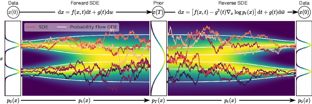
Fig. 2 of Song et al. (2021): the reverse SDE and its probability-flow ODE are the two modes of one sampler (mode="sde" and mode="ode").

diffusion = FlowSampler(model=field, mode="sde", interpolant="vp", prediction="noise")
samples = diffusion.sample(x=torch.randn(1000, 2), n_steps=250)

Optimal-transport couplings

Improving and generalizing flow-based generative models with minibatch optimal transport, Tong et al. 2024. Pair each noise sample with the right datum and the paths straighten, so generation needs fewer steps.

Fig. 1 of Tong et al. (2024): an OT coupling turns crossing, curved transport into straight transport. Same objective, different coupling=.

from torchebm.couplings import SinkhornCoupling, ExactOTCoupling

coupling = SinkhornCoupling(reg=0.05)           # entropic OT; or ExactOTCoupling()
x0, x1 = coupling(x0, x1)                       # re-paired, then interpolate as above

Rectified flow

Flow Straight and Fast, Liu et al. 2023. Retrain on the flow's own (noise, generation) pairs and the trajectories become straight enough for few-step sampling.

Fig. 2 of Liu et al. (2023): paths that cross (left) are rewired by the flow's own pairing into straight ones (right). That rewiring is ReflowCoupling.

from torchebm.couplings import ReflowCoupling

reflow = ReflowCoupling(flow, n_steps=50)       # flow: a trained FlowSampler
x0, x1 = reflow(torch.randn(256, 2))            # x1 = Phi(x0), the model's own output

Contrastive divergence

Training products of experts by minimizing contrastive divergence, Hinton 2002, with the deep-EBM recipe of Du & Mordatch 2019. Push the energy down on data and up on short-run MCMC negatives.

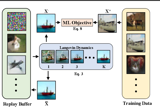
Fig. 1 of Du & Mordatch (2019): Langevin draws the negatives, the buffer persists the chains, the objective separates them from data. That is ContrastiveDivergence(sampler=..., persistent=True).

import torch
from torch import nn
from torchebm.core import BaseModel
from torchebm.datasets import TwoMoonsDataset
from torchebm.losses import ContrastiveDivergence
from torchebm.samplers import LangevinDynamics

class MLPEnergy(BaseModel):                     # E(x): (b, 2) -> (b,)
    def __init__(self):
        super().__init__()
        self.net = nn.Sequential(nn.Linear(2, 128), nn.SiLU(), nn.Linear(128, 1))
    def forward(self, x):
        return self.net(x).squeeze(-1)

data = TwoMoonsDataset(n_samples=3000, noise=0.05).get_data()
energy = MLPEnergy()
sampler = LangevinDynamics(model=energy, step_size=0.1, noise_scale=1.0)

cd = ContrastiveDivergence(model=energy, sampler=sampler, k_steps=10)  # CD-10
opt = torch.optim.Adam(energy.parameters(), lr=1e-3)

for _ in range(1000):
    loss, negatives = cd(data[torch.randint(len(data), (256,))])   # (b, 2)
    opt.zero_grad(); loss.backward(); opt.step()

Persistent CD (Tieleman 2008) is one flag: chains resume from a replay buffer instead of restarting at the data.

cd = ContrastiveDivergence(model=energy, sampler=sampler, k_steps=10,
                           persistent=True, buffer_size=8192)

Score matching

Estimation of non-normalized statistical models by score matching, Hyvärinen 2005. No MCMC at all: fit $\nabla_x \log p_\theta$ directly. Denoising (Vincent 2011) and sliced (Song et al. 2019) variants avoid the Hessian trace.

from torchebm.losses import ScoreMatching, DenoisingScoreMatching, SlicedScoreMatching

loss_fn = ScoreMatching(model=energy, hessian_method="exact")
loss_fn = DenoisingScoreMatching(model=energy, noise_scale=0.1)
loss_fn = SlicedScoreMatching(model=energy, n_projections=5)

loss = loss_fn(data[:256])                      # scalar; no sampler needed

Image-scale backbones

A DiT-style conditional transformer (Peebles & Xie 2023) for energies and velocity fields on images, adaLN-Zero blocks included. LabelClassifierFreeGuidance wraps any label-conditioned model base(x, t, y=...) for classifier-free guidance (Ho & Salimans 2022).

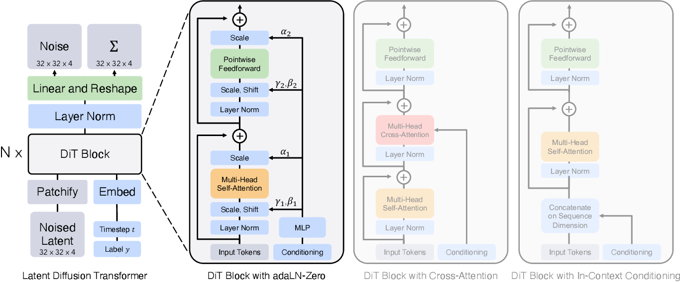
Fig. 3 of Peebles & Xie (2023): the DiT block with adaLN-Zero conditioning, shipped as ConditionalTransformer2D and AdaLNZeroBlock.

from torchebm.models import ConditionalTransformer2D

net = ConditionalTransformer2D(in_channels=3, out_channels=3, input_size=32,
                               patch_size=4, embed_dim=384, depth=12, num_heads=6,
                               cond_dim=10)
out = net(torch.randn(8, 3, 32, 32), cond=torch.randn(8, 10))    # (8, 3, 32, 32)

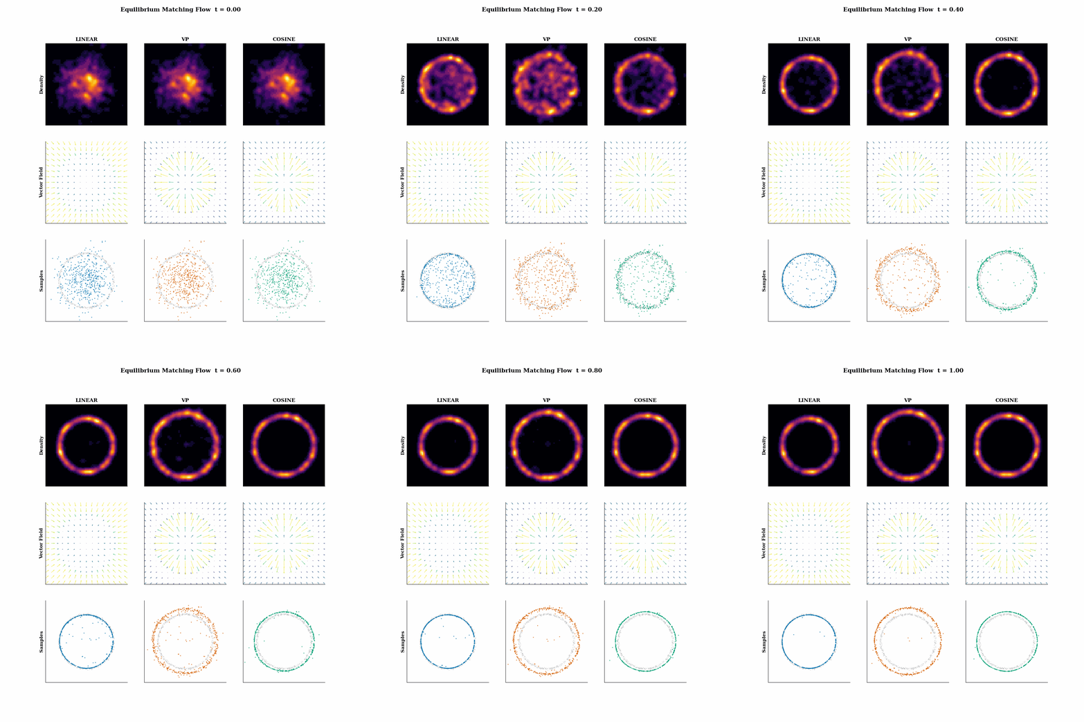
One objective, three interpolants (linear, variance-preserving, cosine): the path changes, the code does not.

Examples

The examples/ tree is a tiered, runnable curriculum, executed in CI so it cannot drift from the library. Browse it on the website.

Tier	You learn to
00-foundations/	work with energies, datasets, schedulers, and interpolants
10-sampling/	sample a fixed target with MCMC, parallel chains, integrators, and flows
20-training/	learn a target: CD, persistent CD, score matching, equilibrium and energy matching, couplings
90-showcase/	study end-to-end demos that push the components

python examples/10-sampling/01-mcmc/01-langevin-101/main.py

Contributing

Contributions are welcome. The Developer Guide covers setup, architecture, and the PR workflow; adding an example is a good first contribution. Check the issues for open tasks, several labelled good first issue.

Show your support for ∇ TorchEBM 🍓

If TorchEBM helps your research, please ⭐️ the repository and spread the word. It genuinely helps others find the project.

Citation

If TorchEBM is useful in your research, please cite it:

@misc{torchebm_library_2025,
  author       = {Ghaderi, Soran and Contributors},
  title        = {{TorchEBM}: A PyTorch Library for Training Energy-Based Models},
  year         = {2025},
  url          = {https://github.com/soran-ghaderi/torchebm},
}

Citations

@article{hinton2002training,
  title   = {Training products of experts by minimizing contrastive divergence},
  author  = {Hinton, Geoffrey E.},
  journal = {Neural Computation},
  volume  = {14},
  number  = {8},
  year    = {2002},
}

@article{hyvarinen2005estimation,
  title   = {Estimation of non-normalized statistical models by score matching},
  author  = {Hyv{\"a}rinen, Aapo},
  journal = {Journal of Machine Learning Research},
  volume  = {6},
  year    = {2005},
}

@article{vincent2011connection,
  title   = {A connection between score matching and denoising autoencoders},
  author  = {Vincent, Pascal},
  journal = {Neural Computation},
  volume  = {23},
  number  = {7},
  year    = {2011},
}

@article{girolami2011riemann,
  title   = {Riemann manifold {L}angevin and {H}amiltonian {M}onte {C}arlo methods},
  author  = {Girolami, Mark and Calderhead, Ben},
  journal = {Journal of the Royal Statistical Society: Series B},
  volume  = {73},
  number  = {2},
  year    = {2011},
}

@inproceedings{song2019sliced,
  title   = {Sliced Score Matching: A Scalable Approach to Density and Score Estimation},
  author  = {Song, Yang and Garg, Sahaj and Shi, Jiaxin and Ermon, Stefano},
  year    = {2019},
  eprint  = {1905.07088},
  url     = {https://arxiv.org/abs/1905.07088},
}

@inproceedings{du2019implicit,
  title   = {Implicit Generation and Generalization in Energy-Based Models},
  author  = {Du, Yilun and Mordatch, Igor},
  year    = {2019},
  eprint  = {1903.08689},
  url     = {https://arxiv.org/abs/1903.08689},
}

@inproceedings{song2021scorebased,
  title   = {Score-Based Generative Modeling through Stochastic Differential Equations},
  author  = {Song, Yang and Sohl-Dickstein, Jascha and Kingma, Diederik P. and Kumar, Abhishek and Ermon, Stefano and Poole, Ben},
  year    = {2021},
  eprint  = {2011.13456},
  url     = {https://arxiv.org/abs/2011.13456},
}

@inproceedings{lipman2023flow,
  title   = {Flow Matching for Generative Modeling},
  author  = {Lipman, Yaron and Chen, Ricky T. Q. and Ben-Hamu, Heli and Nickel, Maximilian and Le, Matt},
  year    = {2023},
  eprint  = {2210.02747},
  url     = {https://arxiv.org/abs/2210.02747},
}

@inproceedings{liu2023flow,
  title   = {Flow Straight and Fast: Learning to Generate and Transfer Data with Rectified Flow},
  author  = {Liu, Xingchao and Gong, Chengyue and Liu, Qiang},
  year    = {2023},
  eprint  = {2209.03003},
  url     = {https://arxiv.org/abs/2209.03003},
}

@article{albergo2023stochastic,
  title   = {Stochastic Interpolants: A Unifying Framework for Flows and Diffusions},
  author  = {Albergo, Michael S. and Boffi, Nicholas M. and Vanden-Eijnden, Eric},
  year    = {2023},
  eprint  = {2303.08797},
  url     = {https://arxiv.org/abs/2303.08797},
}

@article{tong2024improving,
  title   = {Improving and generalizing flow-based generative models with minibatch optimal transport},
  author  = {Tong, Alexander and Fatras, Kilian and Malkin, Nikolay and Huguet, Guillaume and Zhang, Yanlei and Rector-Brooks, Jarrid and Wolf, Guy and Bengio, Yoshua},
  journal = {Transactions on Machine Learning Research},
  year    = {2024},
  eprint  = {2302.00482},
  url     = {https://arxiv.org/abs/2302.00482},
}

@article{wang2025equilibrium,
  title   = {Equilibrium Matching: Generative Modeling with Implicit Energy-Based Models},
  author  = {Wang, Runqian and Du, Yilun},
  year    = {2025},
  eprint  = {2510.02300},
  url     = {https://arxiv.org/abs/2510.02300},
}

@article{balcerak2025energy,
  title   = {Energy Matching: Unifying Flow Matching and Energy-Based Models for Generative Modeling},
  author  = {Balcerak, Michal and Amiranashvili, Tamaz and Terpin, Antonio and Shit, Suprosanna and Bogensperger, Lea and Kaltenbach, Sebastian and Koumoutsakos, Petros and Menze, Bjoern},
  year    = {2025},
  eprint  = {2504.10612},
  url     = {https://arxiv.org/abs/2504.10612},
}

@inproceedings{peebles2023scalable,
  title   = {Scalable Diffusion Models with Transformers},
  author  = {Peebles, William and Xie, Saining},
  year    = {2023},
  eprint  = {2212.09748},
  url     = {https://arxiv.org/abs/2212.09748},
}

@article{debortoli2021diffusion,
  title   = {Diffusion {S}chr{\"o}dinger Bridge with Applications to Score-Based Generative Modeling},
  author  = {De Bortoli, Valentin and Thornton, James and Heng, Jeremy and Doucet, Arnaud},
  year    = {2021},
  eprint  = {2106.01357},
  url     = {https://arxiv.org/abs/2106.01357},
}

Changelog

See CHANGELOG for version history.

License

MIT License. See LICENSE for details.

Research collaboration

If you are interested in collaborating on research around energy-based, flow-based, or diffusion models, feel free to reach out. Contributions to TorchEBM 🍓 and discussions that push the field forward are always welcome.