AMLCS

The AMLCS Package is a FORTRAN+Python based package which holds the following Data Assimilation methods for the SPEEDY model:

1. Szunyogh, I., Kostelich, E. J., Gyarmati, G., Kalnay, E., Hunt, B. R., Ott, E., ... & Yorke, J. A. (2008). A local ensemble transform Kalman filter data assimilation system for the NCEP global model. Tellus A: Dynamic Meteorology and Oceanography, 60(1), 113-130.
2. Anderson, J. L. (2012). Localization and sampling error correction in ensemble Kalman filter data assimilation. Monthly Weather Review, 140(7), 2359-2371.
3. Nino-Ruiz, E. D., Sandu, A., & Deng, X. (2019). A parallel implementation of the ensemble Kalman filter based on modified Cholesky decomposition. Journal of Computational Science, 36, 100654.

If you use this repo, please cite the following papers:

1. Nino-Ruiz, Elías D., and Randy Consuegra. AMLCS-DA: A data assimilation package in Python for Atmospheric General Circulation Models. SoftwareX 22 (2023): 101374.
2. Nino-Ruiz, E. D., Guzman-Reyes, L. G., & Beltran-Arrieta, R. (2020). An adjoint-free four-dimensional variational data assimilation method via a modified Cholesky decomposition and an iterative Woodbury matrix formula. Nonlinear Dynamics, 99(3), 2441-2457.
3. Nino-Ruiz, E. D., Sandu, A., & Deng, X. (2018). An ensemble Kalman filter implementation based on modified Cholesky decomposition for inverse covariance matrix estimation. SIAM Journal on Scientific Computing, 40(2), A867-A886.

Code Documentation

Description

The following code defines several variables and objects necessary for a data assimilation process:

• gs: an instance of grid_resolution class created with res_name parameter.
• data_obs: a string of observed data separated by commas extracted from the err_obs column of df_par dataframe.
• err_obs: a list of floating-point numbers created by converting the values in data_obs.
• plac_obs: a string of observation positions separated by commas extracted from the obs_plc column of df_par dataframe.
• obs_plc: a list of integers created by converting the values in plac_obs.
• ob: an instance of observation class created with err_obs and obs_plc as parameters.
• nm: an instance of numerical_model class created with path_method, gs, Nens, and par parameters.
• rs: an instance of reference_solution class created with nm and M parameters.
• seq_da: an instance of a class that inherits from sequential_method created with nm, infla, Nens, and method parameters.
• em_bck: an instance of error_metric class created with nm, "bck", and M as parameters.
• em_ana: an instance of error_metric class created with nm, "ana", and M as parameters.
• tm_bck: an instance of time_metric class created with nm, "bck", and M as parameters.
• tm_ana: an instance of time_metric class created with nm, "ana", and M as parameters.

Parameters

• res_name: a string that defines the grid resolution.
• df_par: a dataframe that contains observational and model parameters.
• path_method: a string that defines the path to the numerical model.
• Nens: an integer that defines the number of ensemble members.
• par: a dictionary that contains model parameters.
• option_mask: a string that defines the relation between state variables and model parameters.
• exp_settings: a dictionary that contains experimental settings.
• args: a dictionary that contains additional arguments.
• r: a float that defines the sub-domain computation radius.
• M: an integer that defines the number of assimilation cycles.
• infla: a float that defines the inflation factor.
• method: a string that defines the assimilation method.
• s: a float that defines the observational noise standard deviation.
• list_k: a list that contains the assimilation cycle numbers to store.

Example Usage

gs = grid_resolution(res_name);
data_obs = df_par['err_obs'].iloc[0].strip().split(',');
err_obs = [float(v) for v in data_obs];
plac_obs = df_par['obs_plc'].iloc[0].strip().split(',');
obs_plc = [int(v) for v in plac_obs];
ob = observation(err_obs, obs_plc);

nm = numerical_model(path_method, gs, Nens, par=par);
nm.define_relations(option=option_mask);
nm.load_settings(exp_settings, args);
     
gs.create_mesh(nm);
gs.compute_sub_domains(r);
rs = reference_solution(nm, M);
    
seq_da = sequential_method(method).get_instance(nm, infla, Nens);
    
ob.build_observational_network(gs, nm, s=s);
ob.build_synthetic_observations(nm, rs, M); 
    
em_bck = error_metric(nm, 'bck', M);
em_ana = error_metric(nm, 'ana', M);
tm_bck =  time_metric(nm, 'bck');
tm_ana =  time_metric(nm, 'ana');
    
for k in range(0, M):
    seq_da.load_background_ensemble();
        
    tm_bck.start_time();
    seq_da.prepare_background();
    tm_bck.check_time();
        
    tm_ana.start_time();
    seq_da.prepare_analysis(ob, k);
    seq_da.perform_assimilation(ob);
    tm_ana.check_time();
       
    em_bck.compute_error_step(k, seq_da.XB, rs.x_ref[k]);
    em_ana.compute_error_step(k, seq_da.XA, rs.x_ref[k]);
        
    em_bck.store_all_results();
    em_ana.store_all_results();
    tm_bck.store_all_results();
    tm_ana.store_all_results();
        
    seq_da.check_time_store(k, list_k);
        
    seq_da.perform_forecast();

Adding a new model

Incorporating Other DA Algorithms and Dynamical Models in AMLCS-DA Package

The AMLCS-DA package provides a flexible framework for incorporating other data assimilation (DA) algorithms and dynamical models.

Adding a New DA Algorithm

To add a new DA algorithm, you need to create a new class that inherits from the SequentialAlgorithm abstract class. This class should implement the following methods:

• prepare_background(): prepares the background state for assimilation
• prepare_analysis(observation, time_step): prepares the analysis state for assimilation based on the current observation and time step
• perform_assimilation(observation): performs the assimilation step using the current observation
• perform_forecast(): performs the forecast step

Adding a New Dynamical Model

To add a new dynamical model, you need to create a new class that inherits from the NumericalModel abstract class. This class should implement the following methods:

• step_forward(state, time_step): steps forward the model state by the given time step
• define_relations(option): defines the relations between the state variables of the model
• load_settings(settings): loads the settings of the model

Example

Here is an example of how to add a new DA algorithm and dynamical model in the AMLCS-DA package:

from AMLCS.da.sequential_algorithm import SequentialAlgorithm
from AMLCS.da.numerical_model import NumericalModel

class MyAlgorithm(SequentialAlgorithm):
    # Implement the required methods here

class MyModel(NumericalModel):
    # Implement the required methods here

# Instantiate the new DA algorithm and dynamical model
algorithm = MyAlgorithm()
model = MyModel()

# Use the new algorithm and model in the AMLCS-DA package
da_system = AMLCS_DA(algorithm, model)

Adding the Lorenz 96 model to AMLCS-DA:

To add a new dynamical model to the AMLCS-DA package, you need to define the model equations and implement them as a class in the dynamical_model.py file. This class should inherit the abstract class DynamicalModel and implement the following methods:

• __init__(self, n): initialize the model parameters and state with the size n
• integrate(self, t0, tf, dt): integrate the model equations from t0 to tf with time step dt
• get_state(self): return the current state of the model
• set_state(self, state): set the state of the model to state

Once you have defined your new dynamical model class, you can use it in the AMLCS-DA package by specifying it as an argument to the numerical_model constructor. For example, if you have defined a Lorenz96 model in a class called Lorenz96Model, you can use it as follows:

from amlcsda.numerical_model import numerical_model
from my_dynamical_model import Lorenz96Model

# Define the model parameters
path_method = 'EnSRF'
gs = 0.05
Nens = 20
par = {'F': 8.0, 'h': 1.0}

# Create an instance of the Lorenz96 model
model = Lorenz96Model(n=40)

# Create an instance of the numerical model using the Lorenz96 model
nm = numerical_model(path_method, gs, Nens, par=par, dynamical_model=model)

# Run the model
nm.run_model()

In this example, we create an instance of the Lorenz96Model class with n=40 and pass it as an argument to the numerical_model constructor. We then run the model using the run_model method of the numerical_model object.

class Lorenz96Model(DynamicalModel):
    def __init__(self, n):
        self.n = n
        self.F = 8.0
        self.h = 1.0
        self.x = np.zeros(self.n)
        
    def integrate(self, t0, tf, dt):
        # Integration code here
        
    def get_state(self):
        return self.x
    
    def set_state(self, state):
        self.x = state

Class Diagram

The class diagram represents the organization and interconnection of the classes within the AMLCS package. AMLCS is a Python toolbox for testing sequential Data Assimilation (DA) methods using the SPEEDY model, which is a well-known Atmospheric General Circulation model in the DA community.

The classes in the diagram are divided into five categories: grid, numerical model, DA methods, input/output, and plot/covariance. The grid class contains a single Grid class that defines the grid resolution used in the numerical model. The numerical model category includes two classes: NumericalModel and ICTools. NumericalModel is the core class that defines the atmospheric model, while ICTools contains methods for creating initial conditions.

The DA methods category includes four classes: DA, LETKF, LEKF, and ETKF. These classes implement well-known ensemble-based DA methods, such as the Local Ensemble Transform Kalman Filter (LETKF) and the Local Ensemble Kalman Filter (LEKF). The input/output category includes a single IO class that contains methods for reading and writing data. The plot/covariance category includes two classes: PlotTools and Covariance. PlotTools contains methods for visualizing data, while Covariance contains methods for computing the background error covariance matrix.

Finally, the AMLCS package includes three scripts: AMLCS_PRE, AMLCS_MAIN, and AMLCS_POST, which are responsible for performing the preprocessing, assimilation, and post-processing steps, respectively. These scripts utilize the classes defined in the package to perform the various DA operations.

Class definitions

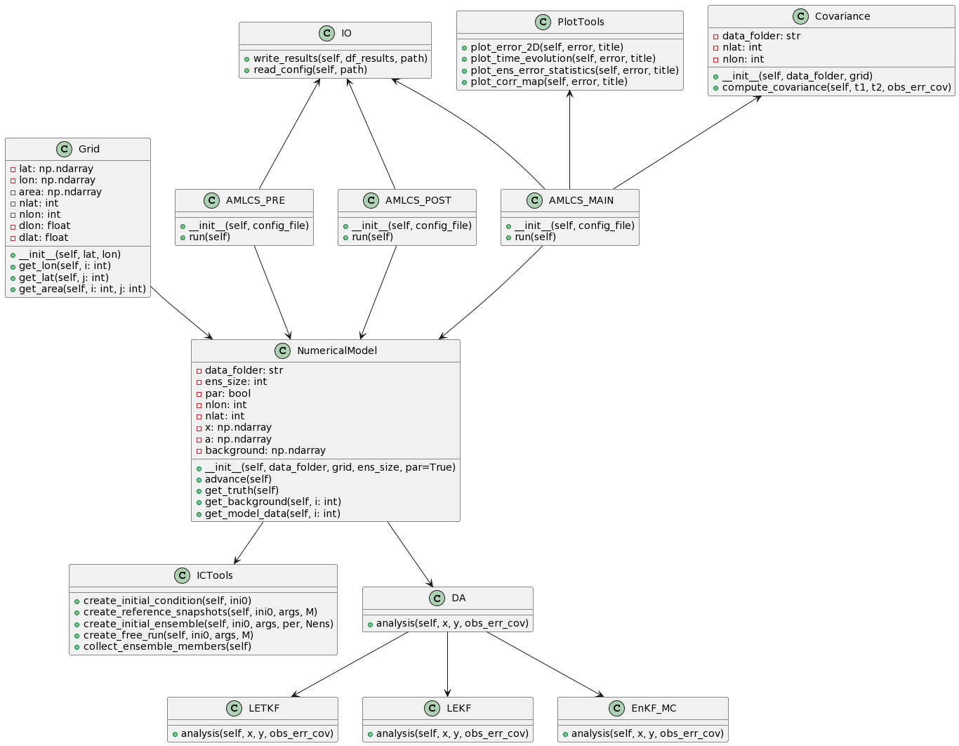
The AMLCS-DA package includes the following classes:

• Grid: Defines the spatial discretization of the domain using a specific grid resolution. It contains information about the domain size, grid spacing, and the number of grid points.
• NumericalModel: Implements the forecast step of the DA cycle using the AT-GCM SPEEDY by default. It is responsible for integrating the model forward in time, creating initial conditions for the ensemble members, and generating the reference trajectory. This class also provides methods for collecting ensemble members, creating free runs, and performing the forecast step of the DA cycle.
• DA: An abstract class that defines the basic structure of a DA method. It contains methods for updating the background state using the observation and the forecast error, and for computing the analysis error covariance matrix.
• LETKF: A class that implements the Local Ensemble Transform Kalman Filter method, which uses the local transformation of the ensemble members to update the background state.
• LEKF: A class that implements the Local Ensemble Kalman Filter method, which updates the background state using the ensemble mean and the perturbations around it.
• IO: A class that provides methods for reading and writing input and output files. It includes methods for reading the configuration file, the observations file, and the output files.
• PlotTools: A class that provides methods for generating plots of the results. It includes methods for plotting the time evolution of the analysis and forecast error, the spatial distribution of the analysis error, and the cross-section of the analysis error at different pressure levels.
• Covariance: A class that defines the background error covariance matrix structure. It includes methods for computing the correlation matrix based on different assumptions about the error structure.
• AMLCS_PRE: A class that defines the preprocessing step of the DA cycle. It reads the configuration file and sets up the initial conditions for the forecast and assimilation steps.
• AMLCS_MAIN: A class that runs the main loop of the DA cycle. It reads the observations file and performs the forecast and assimilation steps for each time step.
• AMLCS_POST: A class that postprocesses the output files. It generates plots of the results and computes the statistics of the analysis error.

The relationships between the classes are as follows:

• Grid is used by NumericalModel to define the spatial discretization of the domain.
• NumericalModel is used by all the DA methods (LETKF, LEKF) to perform the forecast step and generate the initial conditions for the ensemble members.
• LETKF and LEKF inherit from the abstract class DA, which defines the basic structure of a DA method.
• IO is used by AMLCS_PRE and AMLCS_MAIN to read input files and write output files.
• PlotTools is used by AMLCS_MAIN and AMLCS_POST to generate plots of the results.
• Covariance is used by LETKF and LEKF to compute the background error covariance matrix.
• AMLCS_PRE sets up the initial conditions for the forecast and assimilation steps, and AMLCS_MAIN performs the forecast and assimilation steps for each time step. AMLCS_POST postprocesses the output files generated by AMLCS_MAIN.

Sequential Diagram

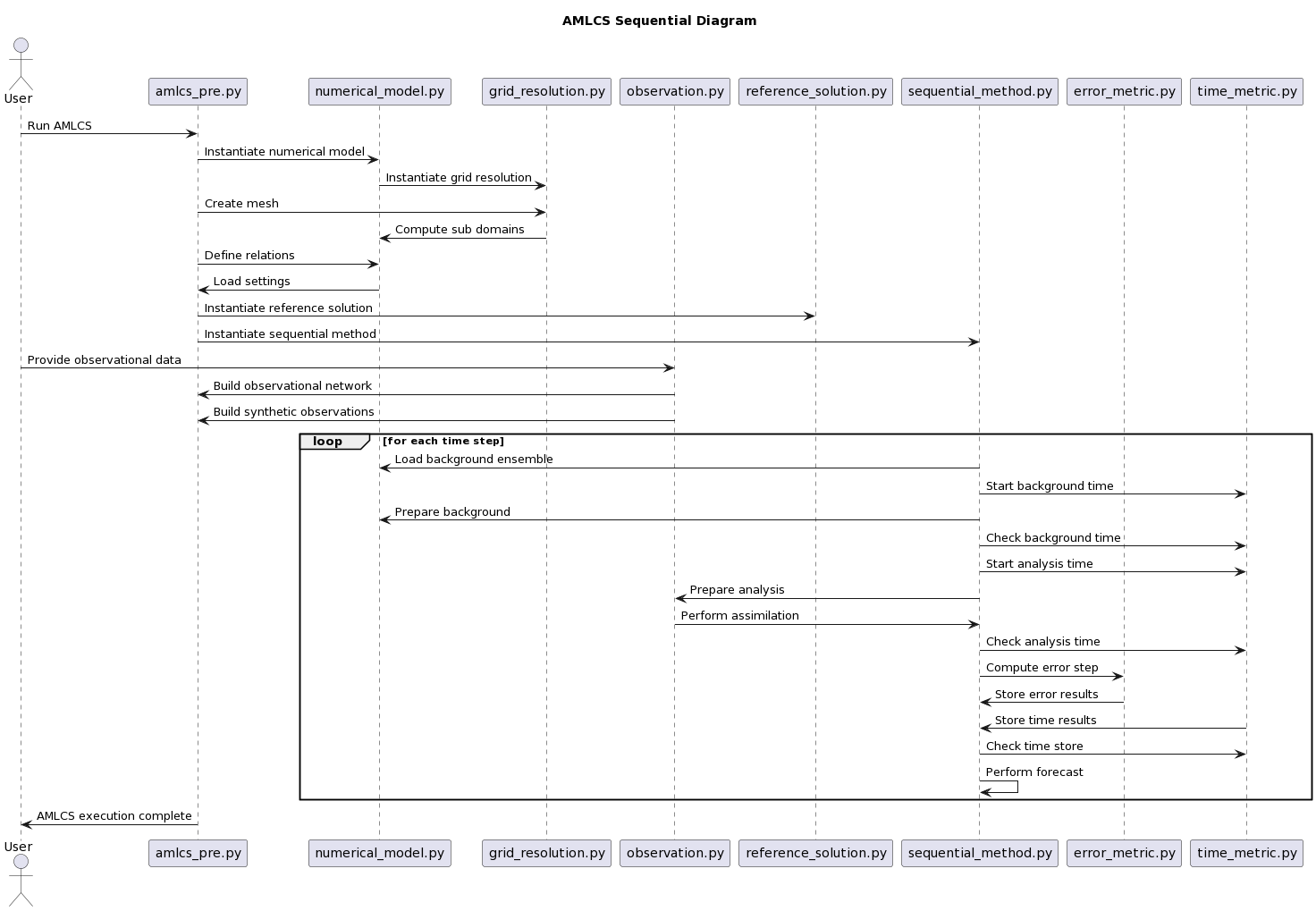
This sequential diagram shows the steps of the AMLCS (Adaptive Multilevel Monte Carlo Localization and Assimilation System) algorithm. The AMLCS algorithm is a data assimilation method used in numerical weather prediction and other fields to combine simulation models and real-world observational data in order to produce more accurate predictions.

The diagram begins with the user running the AMLCS program. The program first instantiates the numerical model (B), which is used to represent the simulated system being studied. The program then instantiates the grid resolution (C) to define the spatial resolution of the model. The grid resolution is then used to create a mesh and compute subdomains for the numerical model.

The program then defines relations between the numerical model and the grid resolution. The program loads the settings for the experiment and instantiates the reference solution (E), which represents the "true" state of the system being simulated. The program also instantiates the sequential method (F), which is used to perform the data assimilation.

Next, the user provides observational data to the program. The observation class (D) is used to build the observational network and generate synthetic observations.

The program then enters a loop for each time step. At each time step, the sequential method loads the background ensemble, prepares the background, and checks the background time. The program then starts the analysis time and prepares the analysis using the observational data. The analysis is then performed by assimilating the observational data into the model using the observation class. The program then checks the analysis time and computes the error step using the error metric class (G). The error results are then stored, along with the time results, using the time metric class (H). The program then checks the time store and performs a forecast for the next time step.

The loop continues until all time steps have been processed. Finally, the program executes the complete AMLCS algorithm and returns the results to the user.

---

Deployment & Reproducibility (Docker)

This section documents how to build a self-contained environment for AMLCS-DA using Docker, and how to run single or batch experiments with automatic timing and per-method logs. It is intended for reproducing the SPEEDY experiments on a fresh Linux machine (local workstation, server, or a cloud VM such as Google Cloud).

Why Docker

The SPEEDY model is compiled with gfortran and links against NetCDF-Fortran. Modern toolchains (gfortran 10+) are stricter than the compiler the code was originally written for, and the Python side pins to numpy<2.0. Docker freezes a known-good environment so the experiments run identically across machines, and avoids the concurrent-I/O issues seen when running the ensemble forecast over a Windows bind-mounted filesystem.

Repository layout expected at run time

AMLCS/
├── Dockerfile
├── run.sh                 # run a single method (with timing)
├── run_all.sh             # run several methods in sequence (auto-Docker)
├── amlcs/                 # Python DA code
├── models/
│   └── speedy/t21/        # SPEEDY Fortran sources + makefile
├── to_run/                # experiment CSV configs and plotting scripts
├── NLD_Paper/             # created at run time (pre-processing + results)
└── logs/                  # created at run time (per-method logs)

Makefile note for modern gfortran

The SPEEDY makefile in models/speedy/t21/ must include the flags -fallow-argument-mismatch -std=legacy so that gfortran 10+ treats the legacy F77 argument-rank mismatches in read_write_netcdf.f as warnings rather than hard errors. The compile flags line should read:

COMOTT1= -O3 -fdefault-real-8 -fconvert=big-endian -frecord-marker=4 -fallow-argument-mismatch -std=legacy

The Dockerfile

The image is based on Ubuntu 22.04 and installs the Fortran toolchain, NetCDF (C and Fortran bindings), and the Python scientific stack. The project itself is NOT copied into the image; it is bind-mounted at run time so that all outputs land on the host disk and persist after the container exits.

FROM ubuntu:22.04

ENV DEBIAN_FRONTEND=noninteractive \
    PYTHONUNBUFFERED=1 \
    LANG=C.UTF-8 \
    LC_ALL=C.UTF-8

RUN apt-get update && apt-get install -y --no-install-recommends \
        build-essential gfortran make git wget curl unzip ca-certificates \
        pkg-config libnetcdf-dev libnetcdff-dev netcdf-bin libhdf5-dev \
        libopenblas-dev liblapack-dev python3 python3-pip python3-dev \
    && rm -rf /var/lib/apt/lists/*

RUN ln -sf /usr/bin/python3 /usr/local/bin/python

RUN pip3 install --no-cache-dir --upgrade pip setuptools wheel \
 && pip3 install --no-cache-dir "numpy<2.0" scipy pandas scikit-learn matplotlib seaborn netCDF4

ENV PROJECT_ROOT=/opt/Research_SPEEDY
WORKDIR ${PROJECT_ROOT}

RUN printf '#!/usr/bin/env bash\nset -e\ncd "${PROJECT_ROOT}"\nif [ -d "${PROJECT_ROOT}/to_run" ] && [ -d "${PROJECT_ROOT}/amlcs" ]; then\n  cp -ru "${PROJECT_ROOT}/to_run/." "${PROJECT_ROOT}/amlcs/"\nfi\ncd "${PROJECT_ROOT}/amlcs"\nexec "$@"\n' > /usr/local/bin/amlcs-entrypoint.sh \
 && chmod +x /usr/local/bin/amlcs-entrypoint.sh

ENTRYPOINT ["/usr/local/bin/amlcs-entrypoint.sh"]
CMD ["bash"]

Build the image once:

cd /path/to/AMLCS
docker build -t amlcs-speedy .

Mapping the project into the container

The entrypoint copies to_run/* into amlcs/ (as the original instructions require) and then drops into amlcs/. The host project directory is mapped to the path the image expects via -v:

docker run --rm -it \
  -v /path/to/AMLCS:/opt/Research_SPEEDY \
  amlcs-speedy bash

Inside the container you are placed in amlcs/ and can run the pipeline by hand:

python3 amlcs_pre.py amlcs_pre_t21.csv     # pre-processing (run once)
python3 amlcs_da.py  amlcs_da_t21_2.csv    # LEnKF
python3 amlcs_da.py  amlcs_da_t21_1.csv    # LETKF
python3 amlcs_da.py  amlcs_da_t21_0.csv    # EnKF_MC_obs

The CSV configuration files

The experiment configs live in to_run/ and amlcs/. The mapping between the provided DA config files and the assimilation method is:

Config file	Method
amlcs_da_t21_0.csv	EnKF_MC_obs
amlcs_da_t21_1.csv	LETKF
amlcs_da_t21_2.csv	LEnKF

Key parameters in the pre-processing config (amlcs_pre_t21.csv):

Parameter	Meaning
Nens	number of ensemble members
M	number of assimilation cycles
res_name	spectral resolution (t21, t30, ...)
per	initial perturbation fraction
obs_steps	model steps between observations
par	enable parallel ensemble forecast (True/False)

Key parameters in the DA config (amlcs_da_t21_*.csv):

Parameter	Meaning
r	local sub-domain radius (box of side 2r+1)
s	observational network spacing (one sensor every s grid points)
method	assimilation method (LEnKF, LETKF, EnKF_MC_obs)
infla	covariance inflation factor
err_obs	per-variable observation error standard deviations
obs_plc	per-variable observation placement flags (which variables are observed)
option_mask	how state variables are grouped into blocks for the covariance
list_snapshots	assimilation cycles for which global snapshots are stored

The pre-processing run produces a directory named {res_name}_{Nens}_{per}_{M} (e.g. t21_80_0.05_30) inside the folder given by folder_prep. All DA methods reuse this same pre-processing directory, so it only needs to be generated once.

Helper script: run.sh

run.sh runs a single method. It auto-detects the project root (so it works from any directory), derives the pre-processing directory name from amlcs_pre_t21.csv, skips pre-processing if it already exists, and reports the wall-clock time of each phase.

./run.sh                      # LEnKF (default)
./run.sh amlcs_da_t21_1.csv   # LETKF
./run.sh amlcs_da_t21_0.csv   # EnKF_MC_obs

Helper script: run_all.sh

run_all.sh runs several methods in sequence. It re-launches itself inside the Docker container automatically (detected via the AMLCS_IN_DOCKER environment variable), so a single command on the host runs the whole batch without typing docker run. Each method writes its own detailed log under logs/, plus a consolidated resumen_<timestamp>.log with the timing of each method.

# from the host, in the project root:
cd /path/to/AMLCS
mkdir -p logs
nohup ./run_all.sh > logs/run_all_master.log 2>&1 &

Monitor progress:

tail -f logs/run_all_master.log     # high-level progress + final summary
tail -f logs/LETKF_*.log            # detailed log of a given method

The methods run strictly sequentially (one finishes before the next starts), while the 80-member ensemble forecast inside each method still runs in parallel when par=True.

Outputs

For each method, a directory named {prep_name}_{method}_{r}_{s}_{infla}_mask_{option_mask} is created under folder_prep. It contains:

• results/ : per-variable RMSE for background (*_bck.csv) and analysis (*_ana.csv), one row per assimilation cycle, one column per pressure level.
• time_snapshots/ : global mean states xb{k}.nc / xa{k}.nc for the cycles listed in list_snapshots.
• timing files time_bck.csv / time_ana.csv with the cost per cycle.

These CSV files feed the plotting scripts in to_run/ (error_comparison_plots.py, error_plots.py, earth_plot.py, etc.).

Running on a cloud VM (e.g. Google Cloud)

On a native Linux VM the concurrent-I/O problem does not occur, so the parallel ensemble forecast (par=True) can be used safely. Typical workflow:

# 1. clone and patch the makefile
git clone https://github.com/enino84/AMLCS.git
cd AMLCS/models/speedy/t21
sed -i 's|^COMOTT1=.*-frecord-marker=4$|COMOTT1= -O3 -fdefault-real-8 -fconvert=big-endian -frecord-marker=4 -fallow-argument-mismatch -std=legacy|' makefile
cd ../../..

# 2. build the image
docker build -t amlcs-speedy .

# 3. run all methods in the background, with logs
mkdir -p logs
nohup ./run_all.sh > logs/run_all_master.log 2>&1 &

Because the run is launched with nohup and the heavy work executes inside a detached Docker container, closing the SSH session does not stop the experiment. Reconnect later and inspect logs/ or NLD_Paper/ for results.

Troubleshooting

• ModuleNotFoundError: No module named 'pandas' — the script was run on the host instead of inside the container. Run it through Docker (or use run_all.sh, which enters Docker automatically).
• Fortran runtime error: End of file in cpl_land.f during the forecast — concurrent reads/writes of the per-member restart files corrupted them. This happens on bind-mounted non-native filesystems (e.g. Docker Desktop on Windows). Use a native Linux filesystem, or set par=False in amlcs_pre_t21.csv to force a sequential ensemble forecast.
• Rank mismatch warnings while compiling SPEEDY — harmless; produced by the legacy F77 NetCDF calls and silenced to warnings by -fallow-argument-mismatch.
• rm: cannot remove '*.ctl' — harmless; the SPEEDY compile.sh performs a pre-emptive cleanup before files exist.