start_here.py

"""
PyAutoLens
==========

**PyAutoLens** is software for analysing strong gravitational lenses, an astrophysical phenomenon where a galaxy
appears multiple times because its light is bent by the gravitational field of an intervening foreground lens galaxy.

Here is a schematic of a strong gravitational lens:

![Schematic of Gravitational Lensing](https://raw.githubusercontent.com/PyAutoLabs/PyAutoLens/main/docs/overview/images/overview_1_lensing/schematic.jpg)
**Credit: F. Courbin, S. G. Djorgovski, G. Meylan, et al., Caltech / EPFL / WMKO**
https://www.astro.caltech.edu/~george/qsolens/

This notebook gives a starting overview of **PyAutoLens**'s features and API.

__Google Colab Setup__

The introduction `start_here` examples are available on Google Colab, which allows you to run them in a web browser
without manual local PyAutoLens installation.

The code below sets up your environment if you are using Google Colab, including installing autolens and downloading
files required to run the notebook. If you are running this script not in Colab (e.g. locally on your own computer),
running the code will still check correctly that your environment is set up and ready to go.
"""

import subprocess
import sys

try:
    import google.colab

    subprocess.check_call(
        [sys.executable, "-m", "pip", "install", "autoconf", "--no-deps"]
    )
except ImportError:
    pass

from autoconf import setup_colab

setup_colab.for_autolens(
    raise_error_if_not_gpu=False  # Switch to False for CPU Google Colab
)

"""
__Imports__

Lets first import autolens, its plotting module and the other libraries we'll need.

You'll see these imports in the majority of workspace examples.
"""
# %matplotlib inline

from pathlib import Path
import matplotlib.pyplot as plt

import autolens as al
import autoarray as aa
import autolens.plot as aplt

"""
Lets illustrate a simple gravitational lensing calculation, creating an an image of a lensed galaxy using a 
light profile and mass profile.

__Grid__

The emission of light from a source galaxy, which is gravitationally lensed around the lens galaxy, is described 
using the `Grid2D` data structure, which is two-dimensional Cartesian grids of (y,x) coordinates.

We make and plot a uniform Cartesian grid:
"""
grid = al.Grid2D.uniform(
    shape_native=(150, 150),  # The [pixels x pixels] shape of the grid in 2D.
    pixel_scales=0.05,  # The pixel-scale describes the conversion from pixel units to arc-seconds.
)

aplt.plot_grid(grid=grid, title="")

"""
__Light Profiles__

Our aim is to create an image of the source galaxy after its light has been deflected by the mass of the foreground
lens galaxy. We therefore need to ray-trace the `Grid2D`'s coordinates from the 'image-plane' to the 'source-plane'.

This uses analytic functions representing a galaxy's light and mass distributions, referred to as `LightProfile` and
`MassProfile` objects.

The most common light profile in Astronomy is the elliptical Sersic, which we create an instance of below:
"""
sersic_light_profile = al.lp.Sersic(
    centre=(0.0, 0.0),  # The light profile centre [units of arc-seconds].
    ell_comps=(
        0.2,
        0.1,
    ),  # The light profile elliptical components [can be converted to axis-ratio and position angle].
    intensity=0.005,  # The overall intensity normalisation [units arbitrary and are matched to the data].
    effective_radius=2.0,  # The effective radius containing half the profile's total luminosity [units of arc-seconds].
    sersic_index=4.0,  # Describes the profile's shape [higher value -> more concentrated profile].
)

"""
By passing the light profile the `grid`, we evaluate the light emitted at every (y,x) coordinate and therefore create 
an image of the Sersic light profile.
"""
image = sersic_light_profile.image_2d_from(grid=grid)

plt.imshow(image.native.array)  # Dont worry about the use of .native.array for now.

"""
__Plotting__

In-built plotting methods are provided for plotting objects and their properties, like the image of
a light profile we just created.

By using a `aplt.plot_array` to plot the light profile's image, the figured is improved. 

Its axis units are scaled to arc-seconds, a color-bar is added, its given a descriptive labels, etc.

The plot module is highly customizable and designed to make it straight forward to create clean and informative figures
for fits to large datasets.
"""
aplt.plot_array(array=sersic_light_profile.image_2d_from(grid=grid), title="Image")

"""
__Mass Profiles__

PyAutoLens uses MassProfile objects to represent a galaxy’s mass distribution and perform ray-tracing calculations.

Below we create an elliptical isothermal MassProfile and compute its deflection angles on our Cartesian grid, where 
the deflection angles describe how the lens galaxy’s mass bends the source’s light:
"""
isothermal_mass_profile = al.mp.Isothermal(
    centre=(0.0, 0.0),  # The mass profile centre [units of arc-seconds].
    ell_comps=(
        0.1,
        0.0,
    ),  # The mass profile elliptical components [can be converted to axis-ratio and position angle].
    einstein_radius=1.6,  # The Einstein radius [units of arc-seconds].
)

deflections = isothermal_mass_profile.deflections_yx_2d_from(grid=grid)

"""
The deflection angles are easily plotted using the **PyAutoLens** plot module.

(Many other lensing quantities are also easily plotted, for example the `convergence` and `potential`).
"""
deflections = isothermal_mass_profile.deflections_yx_2d_from(grid=grid)
deflections_y = aa.Array2D(values=deflections.slim[:, 0], mask=grid.mask)
aplt.plot_array(array=deflections_y, title="Deflections Y")
deflections = isothermal_mass_profile.deflections_yx_2d_from(grid=grid)
deflections_x = aa.Array2D(values=deflections.slim[:, 1], mask=grid.mask)
aplt.plot_array(array=deflections_x, title="Deflections X")
aplt.plot_array(
    array=isothermal_mass_profile.convergence_2d_from(grid=grid), title="Convergence"
)
aplt.plot_array(
    array=isothermal_mass_profile.potential_2d_from(grid=grid), title="Potential"
)

"""
__Galaxy__

A `Galaxy` object is a collection of light profiles at a specific redshift.

This object is highly extensible and is what ultimately allows us to fit complex models to strong lens images.

We create two galaxies representing the lens and source galaxies shown in the strong lensing diagram above.
"""
lens_galaxy = al.Galaxy(
    redshift=0.5,
    light=sersic_light_profile,  # The foreground lens's light is typically observed in a strong lens.
    mass=isothermal_mass_profile,  # Its mass is what causes the strong lensing effect.
)

source_light_profile = al.lp.Exponential(
    centre=(
        0.3,
        0.2,
    ),  # The source galaxy's light is observed, appearing as multiple images around the lens galaxy.
    ell_comps=(
        0.1,
        0.0,
    ),  # However, the mass of the source does not impact the strong lensing effect.
    intensity=0.1,  # and is not included.
    effective_radius=0.5,
)

source_galaxy = al.Galaxy(redshift=1.0, light=source_light_profile)

"""
The `aplt.plot_array` function plots properties of the lens and source galaxies.
"""
aplt.plot_array(array=lens_galaxy.image_2d_from(grid=grid), title="Lens Galaxy Image")
aplt.plot_array(
    array=source_galaxy.image_2d_from(grid=grid), title="Source Galaxy Image"
)

"""
__Tracer__

The `Tracer` object is a collection of galaxies at different redshifts (often referred to as planes). 

It uses these galaxies to perform ray-tracing, using the mass profiles of the galaxies to bend the light of the source
galaxy(s) into the multiple images we observe in a strong lens system. 

This is shown below, where the image of the tracer shows a distinct Einstein ring of the source galaxy.
"""
tracer = al.Tracer(galaxies=[lens_galaxy, source_galaxy], cosmology=al.cosmo.Planck15())

image = tracer.image_2d_from(grid=grid)

aplt.plot_array(array=tracer.image_2d_from(grid=grid), title="Image")

"""
__JAX__

**PyAutoLens** runs on either **NumPy** (the default) or **JAX** (Google's
array library with GPU support and just-in-time compilation). JAX makes
lens modeling 10-100x faster on large grids — sometimes more on GPU — so
the library is built to use it automatically wherever it helps.

You do not have to do anything to opt in. If you installed `autolens` with
the JAX extra (`pip install autolens[jax]` on Python 3.11+), the
`AnalysisImaging`, `AnalysisInterferometer`, and `AnalysisPoint` classes
you'll meet in the `__Lens Modeling__` section below default to
`use_jax=True`. The non-linear search driver (Nautilus, dynesty, ...)
batches parameter vectors and evaluates the likelihood through
`jax.vmap(jax.jit(...))` internally. You'll see a one-time log line like
`JAX: Applying vmap and jit to likelihood function -- may take a few
seconds.` the first time a search starts; that's the JIT compile kicking
in, after which evaluations re-use the compiled trace.

If JAX is not installed, the analysis warns once and falls back to NumPy
automatically. You can force NumPy explicitly with
`al.AnalysisImaging(dataset=dataset, use_jax=False)` or by setting
`PYAUTO_DISABLE_JAX=1` — useful when debugging, where NumPy stack traces
are easier to read than JAX traces.

__When you write `@jax.jit` yourself__

Two situations call for it:

1. **Custom simulations.** Pass `use_jax=True` to the simulator constructor
   and wrap your call in `@jax.jit` when you want to render many datasets
   fast — parameter sweeps, mock-data studies, batch figure generation.
   For example:

   ```python
   import jax

   simulator = al.SimulatorImaging(
       exposure_time=300.0, psf=psf, background_sky_level=0.1, use_jax=True
   )

   @jax.jit
   def simulate(tracer):
       return simulator.via_tracer_from(tracer=tracer, grid=grid)
   ```

   The per-dataset-type `simulator.py` scripts (`scripts/imaging/simulator.py`,
   `scripts/interferometer/simulator.py`, `scripts/point_source/simulator.py`)
   each show the canonical pattern in their `__JAX Variant__` section.

2. **Custom likelihood functions** that you assemble by hand rather than
   reaching for `AnalysisImaging`. Same shape: `@jax.jit` around your own
   `def log_likelihood(instance): ...` that builds a `Tracer` and a
   `FitImaging` and returns `fit.log_likelihood`. See the per-dataset-type
   `likelihood_function.py` scripts.

For the advanced path — JIT-ing library methods directly (`tracer.image_2d_from`,
`LensCalc.magnification_2d_via_hessian_from`, etc.) without going through a
`Simulator` or `Analysis` — see the `lens_calc.py` workspace guide
(`scripts/guides/lens_calc.py`). That covers the "JIT-it-yourself" pattern,
including the one-time `autolens.jax.register_tracer_classes(tracer)` call
the user makes before the first `@jax.jit`.

__Return-type contract__

When `use_jax=True`, the data structures you get back (`Imaging`, `FitImaging`,
`Tracer.image_2d_from(...)` results, ...) carry `jax.Array` data inside
instead of `numpy.ndarray`. For nearly everything you'd do in a workspace —
plotting, saving to `.fits`, comparing fit residuals — this is transparent:
the plotters and FITS writers call `numpy.asarray()` internally and you see
the same images and numbers you would on the NumPy path.

What changes:

- Arithmetic on JAX arrays stays on the JAX path. Direct calls into NumPy
  (`np.sqrt(fit.residual_map.array)`) will host-transfer the array off the
  GPU; not wrong, but slower than `jnp.sqrt(...)` if you're inside a hot
  loop. For one-off analysis code, don't worry about it.
- The `.array` property of `aa.Array2D` etc. is the raw backing array — a
  `numpy.ndarray` on the NumPy path, a `jax.Array` on the JAX path.

The `data_structures.py` guide (`scripts/guides/data_structures.py`) covers
the wrapper-vs-raw-array distinction in detail.
"""

"""
__Units__

The units used throughout the strong lensing literature vary, therefore lets quickly describe the units used in
**PyAutoLens**.

The `Tracer` object and all mass profiles describe their quantities in terms of angles, which are defined in units
of arc-seconds. To convert these to physical units (e.g. kiloparsecs), we use the redshift of the lens and source
galaxies and an input cosmology. A run through of all normal unit conversions is given in guides in the workspace
outlined below.

The use of angles in arc-seconds has an important property, it means that for a two-plane strong lens system 
(e.g. a lens galaxy at one redshift and source galaxy at another redshift) lensing calculations are independent of
the galaxies' redshifts and the input cosmology. This has a number of benefits, for example it makes it straight
forward to compare the lensing properties of different strong lens systems even when the redshifts of the galaxies
are unknown.

Multi-plane lensing is when there are more than two planes. The tracer fully supports this, if you input 3+ galaxies
with different redshifts into the tracer it will use their redshifts and its cosmology to perform multi-plane lensing
calculations that depend on them.

__Extensibility__

All of the objects we've introduced so far are highly extensible, for example a tracer can be made of many galaxies, a 
galaxy can be made up of any number of light profiles and many galaxy objects can be combined into a galaxies object.

Below, wecreate a `Tracer` with 3 galaxies at 3 different redshifts, forming a system with two distinct Einstein
rings! The mass distribution of the first galaxy has separate components for its stellar mass and dark matter, where
the stellar components use a `LightAndMassProfile` via the `lmp` module.
"""
lens_galaxy_0 = al.Galaxy(
    redshift=0.5,
    bulge=al.lmp.Sersic(
        centre=(0.0, 0.0),
        ell_comps=(0.0, 0.05),
        intensity=0.5,
        effective_radius=0.3,
        sersic_index=3.5,
        mass_to_light_ratio=0.6,
    ),
    disk=al.lmp.Exponential(
        centre=(0.0, 0.0),
        ell_comps=(0.0, 0.1),
        intensity=1.0,
        effective_radius=2.0,
        mass_to_light_ratio=0.2,
    ),
    dark=al.mp.NFWSph(centre=(0.0, 0.0), kappa_s=0.08, scale_radius=30.0),
)

lens_galaxy_1 = al.Galaxy(
    redshift=1.0,
    bulge=al.lp.Exponential(
        centre=(0.00, 0.00),
        ell_comps=(0.05, 0.05),
        intensity=1.2,
        effective_radius=0.1,
    ),
    mass=al.mp.Isothermal(
        centre=(0.0, 0.0), ell_comps=(0.05, 0.05), einstein_radius=0.6
    ),
)

source_galaxy = al.Galaxy(
    redshift=2.0,
    bulge=al.lp.Sersic(
        centre=(0.0, 0.0),
        ell_comps=(0.0, 0.111111),
        intensity=0.7,
        effective_radius=0.1,
        sersic_index=1.5,
    ),
)

tracer = al.Tracer(galaxies=[lens_galaxy_0, lens_galaxy_1, source_galaxy])

aplt.plot_array(array=tracer.image_2d_from(grid=grid), title="Image")

"""
__Lens Modeling__

Lens modeling is the process of fitting a physical model to strong-lensing data in order to infer the properties of
the lens and source galaxies.

The primary goal of **PyAutoLens** is to make lens modeling **simple, scalable to large datasets, and fast**, with
GPU acceleration provided via JAX.

The animation below illustrates the lens modeling workflow. Many models are fitted to the data iteratively,
progressively improving the quality of the fit until the model closely reproduces the observed image.

![Lens Modeling Animation](https://github.com/Jammy2211/auto_files/blob/main/lensmodel.gif?raw=true "model")

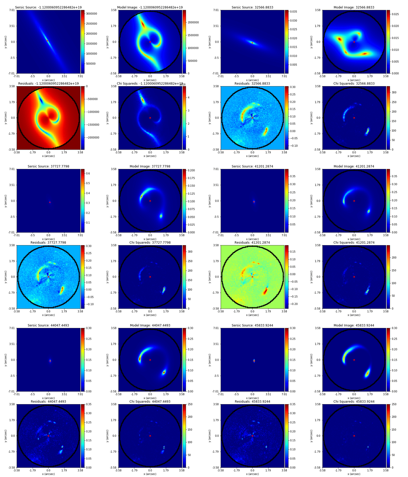
**Credit: Amy Etherington**

The next documentation page guides you through lens modeling for a variety of lensing regimes (e.g. galaxy–galaxy lenses,
cluster-scale lenses) and data types (e.g. CCD imaging, interferometer data).

__Simulations__

Simulating strong lenses is often essential, for example to:

- Practice lens modeling before working with real data.
- Generate large training sets (e.g. for machine learning).
- Test lensing theory in a fully controlled environment.

The next documentation page guides you through how to simulate lenses for different types of strong 
lenses (e.g. galaxy–galaxy lenses, cluster-scale lenses) and different types of data (e.g. CCD imaging, interferometer data).

__Wrap Up__

This completes the introduction to **PyAutoLens**, including a brief overview of the core API for lensing calculations,
lens modeling, and data simulation.

__Where To Next__

**PyAutoLens** can analyse strong lens systems across a range of physical scales (e.g. galaxy, group, and cluster) and for 
different types of data (e.g. imaging, interferometer, and point-source observations). Depending on the scientific 
questions you are interested in, the analysis you perform may differ significantly.

The autolens_workspace contains a suite of example Jupyter Notebooks, organised by lens scale and dataset type.

__Three Ways To Learn PyAutoLens__

There are three ways to learn how to use **PyAutoLens**, which you are free to mix and match:

1. **Manual Navigation**: Read the workspace guides yourself. To find the example notebook best suited to your science
   case, work through the two questions below ("What Scale Lens?" and "What Data Type?"), which point you to the right
   starting point. This is the traditional route, and the rest of this guide supports it.

2. **AI Chat Assistant**: Ask questions to a conversational AI assistant such as ChatGPT or Claude in the browser.
   Point it at the autolens_assistant repository (https://github.com/PyAutoLabs/autolens_assistant) and ask questions
   like "How do I model a galaxy-scale strong lens observed with Hubble imaging?". This is ideal for learning the API,
   working out how to perform a calculation, and interpreting or debugging errors.

3. **Fully Agentic AI**: Use an agentic coding tool such as Claude Code (https://claude.com/claude-code) or Codex
   (https://developers.openai.com/codex) together with autolens_assistant (https://github.com/PyAutoLabs/autolens_assistant).
   These can inspect your data, write and run scripts, and manage an end-to-end lens modeling project directly on your
   machine. See the autolens_assistant repository for more information.

The rest of this guide supports **manual navigation**: we begin by answering two simple questions to find your most
appropriate starting point.

__What Scale Lens?__

What size and scale of strong lens system are you expecting to work with? 

There are three scales to choose from:

- **Galaxy Scale**: Made up of a single lens galaxy lensing a single source galaxy, the simplest strong lens you can get!
  If you're interested in galaxy scale lenses, go to the question below called "What Data Type?".
  
- **Group Scale**: Strong Lens Groups contains 2-10 lens galaxies, normally with one main large galaxy responsible for the majority of lensing.
  They also typically lens just one source galaxy. If you are interested in groups, go to the `group/start_here.ipynb` notebook.
  
- **Cluster Scale**: Strong Lens Galaxy clusters often contained 20-50, or more, lens galaxies, lensing 10, or more, sources galaxies.
  If you are interested in clusters, go to `cluster/start_here.ipynb` notebook.

__What Data Type?__

If you are interested in galaxy-scale strong lenses, you now need to decide what type of strong lens data you are
interested in:

- **CDD Imaging**: For image data from telescopes like Hubble and James Webb, go to `imaging/start_here.ipynb`.

- **Interferometer**: For radio / sub-mm interferometer from instruments like ALMA, go to `interferometer/start_here.ipynb`.

- **Point Sources**: For strongly lensed point sources (e.g. lensed quasars, supernovae), go to `point_source/start_here.ipynb`.

__Google Colab__

You can also open and run each notebook directly in Google Colab, which provides a free cloud computing
environment with all the required dependencies already installed. 

This is a great way to get started quickly without needing to install **PyAutoLens** on your own machine,
so you can check its the right software for you before going through the installation process:

 - [imaging/start_here.ipynb](https://colab.research.google.com/github/PyAutoLabs/autolens_workspace/blob/2026.7.9.1/notebooks/imaging/start_here.ipynb): Galaxy scale strong lenses observed with CCD imaging (e.g. Hubble, James Webb).
 - [interferometer/start_here.ipynb](https://colab.research.google.com/github/PyAutoLabs/autolens_workspace/blob/2026.7.9.1/notebooks/interferometer/start_here.ipynb): Galaxy scale strong lenses observed with interferometer data (e.g. ALMA).
 - [point_source/start_here.ipynb](https://colab.research.google.com/github/PyAutoLabs/autolens_workspace/blob/2026.7.9.1/notebooks/point_source/start_here.ipynb): Galaxy scale strong lenses with a lensed point source (e.g. lensed quasars).
 - [group/start_here.ipynb](https://colab.research.google.com/github/PyAutoLabs/autolens_workspace/blob/2026.7.9.1/notebooks/group/start_here.ipynb): Group scale strong lenses where there are 2-10 lens galaxies.
 - [cluster/start_here.ipynb](https://colab.research.google.com/github/PyAutoLabs/autolens_workspace/blob/2026.7.9.1/notebooks/cluster/start_here.ipynb): Cluster scale strong lenses with 2+ lenses and 5+ source galaxies.

__Still Unsure?__

Each notebook is short and self-contained, and can be completed and adapted quickly to your particular task. 
Therefore, if you're unsure exactly which scale of lensing applies to you, or quite what data you want to use, you 
should just read through a few different notebooks and go from there.

__HowToLens Lectures__

If the start_here examples move too quickly — or you want a slower, more detailed grounding in strong lensing and lens
modeling — **HowToLens** is a separate four-chapter tutorial lecture series written for undergraduates, new PhD
students, or anyone new to the field. It lives in its own repository: https://github.com/PyAutoLabs/HowToLens.

The recommendation is you first look at the start_here example relevant to your science, then go through the lectures
to understand the concepts in more detail.

__Features__

Here is a brief overview of the advanced features of **PyAutoLens**. 

You won't look at these for a while, you should find your relevant start_here notebook and work through that first,
but a quick look through these will give you a sense of the breadth of **PyAutoLens**'s capabilities.

Brief one sentence descriptions of each feature are given, with more detailed descriptions below including 
links to the relevant workspace examples.

**Pixelizations**: Reconstructing the source galaxy on a mesh of pixels, to capture irregular structures like spiral arms.
**Point Sources**: Modeling point sources (e.g. quasars) observed in the strong lens imaging data.
**Interferometry**: Modeling of interferometer data (e.g. ALMA, LOFAR) directly in the uv-plane.
**Multi Gaussian Expansion (MGE)**: Decomposing the lens galaxy into hundreds of Gaussians, for a clean lens subtraction.
**Groups**: Modeling group-scale strong lenses with multiple lens galaxies and multiple source galaxies.
**Multi-Wavelength**: Simultaneous analysis of imaging and / or interferometer datasets observed at different wavelengths.
**Ellipse Fitting**: Fitting ellipses to determine a lens galaxy's ellipticity, position angle and centre.
**Shapelets**: Decomposing a galaxy into a set of shapelet orthogonal basis functions, capturing more complex structures than simple light profiles.
**Operated Light Profiles**: Assuming a light profile has already been convolved with the PSF, for when the PSF is a significant effect.
**Sky Background**: Including the background sky in the model to ensure robust fits to the outskirts of galaxies.

__Pixelizations__

pixelizations reconstruct the source galaxy's light on a pixel-grid. Unlike `LightProfile`'s, they are able to
reconstruct the light of non-symmetric, irregular and clumpy sources.

The image below shows a pixelized source reconstruction of the strong lens SLACS1430+4105, where the source is
reconstructed on a Voronoi mesh adapted to the source morphology, revealing it to be a grand-design face on spiral
galaxy:

![Pixelized Source](https://github.com/PyAutoLabs/PyAutoLens/blob/main/files/imageaxis.png?raw=true)

A complete overview of pixelized source reconstructions can be found
at `notebooks/overview/overview_5_pixelizations.ipynb`.

Chapter 4 of lectures describes pixelizations in detail and teaches users how they can be used to 
perform lens modeling.

__Point Sources__

There are many lenses where the background source is not extended but is instead a point-source, for example strongly
lensed quasars and supernovae.

For these objects, we do not want to model the source using a light profile, which implicitly assumes an extended
surface brightness distribution. 

Instead, we assume that our source is a point source with a centre (y,x), and ray-trace triangles at iteratively
higher resolutions to determine the source's exact locations in the image-plane:

<img src="https://raw.githubusercontent.com/PyAutoLabs/PyAutoLens/main/docs/overview/images/overview_3/point_0.png" width="200">
<img src="https://raw.githubusercontent.com/PyAutoLabs/PyAutoLens/main/docs/overview/images/overview_3/point_1.png" width="200">
<img src="https://raw.githubusercontent.com/PyAutoLabs/PyAutoLens/main/docs/overview/images/overview_3/point_2.png" width="200">
<img src="https://raw.githubusercontent.com/PyAutoLabs/PyAutoLens/main/docs/overview/images/overview_3/point_3.png" width="200">
<img src="https://raw.githubusercontent.com/PyAutoLabs/PyAutoLens/main/docs/overview/images/overview_3/point_4.png" width="200">

Note that the image positions above include the fifth central image of the strong lens, which is often not seen in 
strong lens imaging data. It is easy to disable this image in the point source modeling.

Checkout the`autolens_workspace/*/point_source` package to get started.

__Interferometry__

Modeling of interferometer data from submillimeter (e.g. ALMA) and radio (e.g. LOFAR) observatories:

![ALMA Image](https://raw.githubusercontent.com/PyAutoLabs/PyAutoGalaxy/main/paper/almacombined.png)

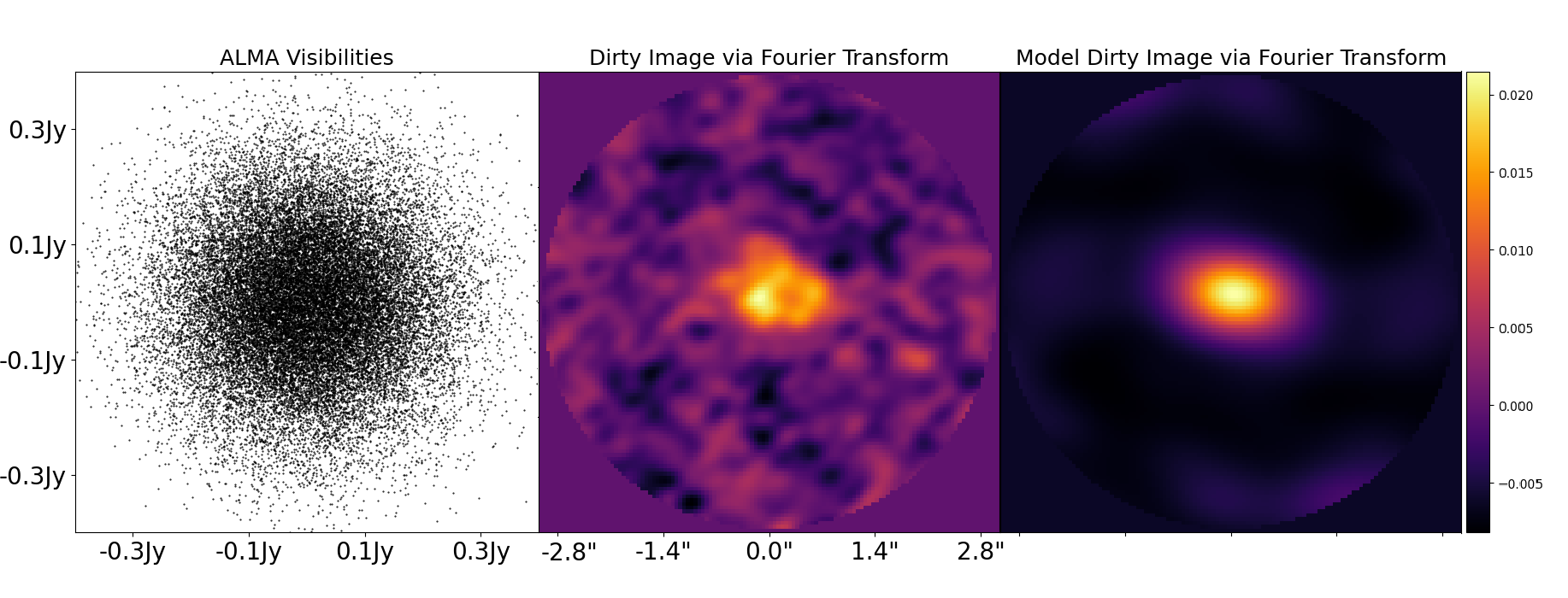
Visibilities data is fitted directly in the uv-plane, circumventing issues that arise when fitting a dirty image
such as correlated noise. This uses the non-uniform fast fourier transform algorithm
[PyNUFFT](https://github.com/jyhmiinlin/pynufft) to efficiently map the galaxy model images to the uv-plane.

Checkout the`autolens_workspace/*/interferometer` package to get started.


__Multi Gaussian Expansion (MGE)__

An MGE decomposes the light of a galaxy into tens or hundreds of two dimensional Gaussians:

![MGE](https://raw.githubusercontent.com/PyAutoLabs/PyAutoLens/main/docs/overview/images/overview_3/mge.png)

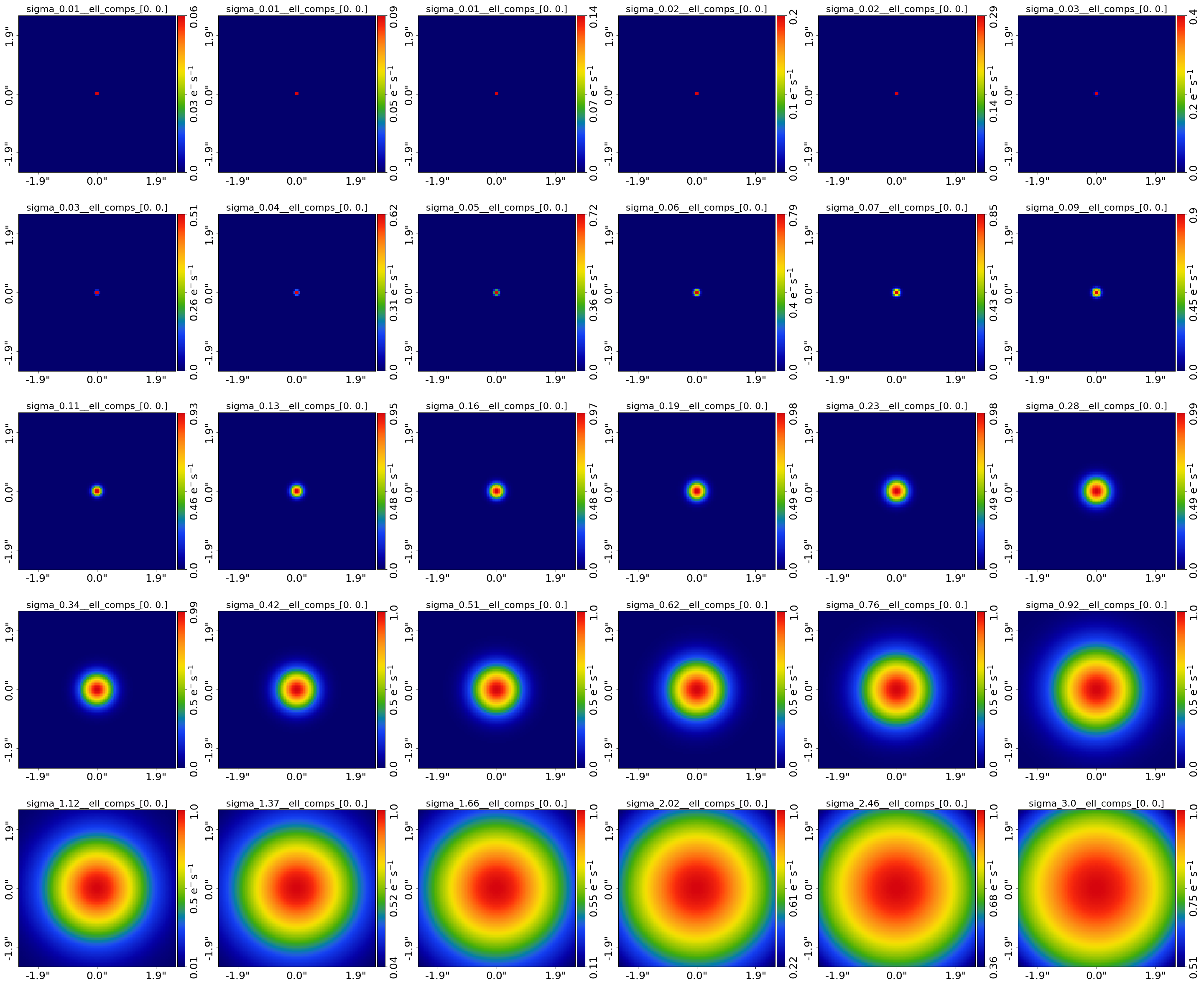
In the image above, 30 Gaussians are shown, where their sizes go from below the pixel scale (in order to resolve
point emission) to beyond the size of the galaxy (to capture its extended emission).

It is an extremely powerful way to model and subtract the light of the foreground lens galaxy in strong lens imaging,
and makes it possible to model the stellar mass of the lens galaxy in a way that is tied to its light.

Scientific Applications include capturing departures from elliptical symmetry in the light of galaxies, providing a 
flexible model to deblend the emission of point sources (e.g. quasars) from the emission of their host galaxy and 
deprojecting the light of a galaxy from 2D to 3D.

The following paper gives a detailed overview of MGEs and their applications in strong lensing: https://arxiv.org/abs/2403.16253

Checkout `autolens_workspace/notebooks/features/multi_gaussian_expansion.ipynb` to learn how to use an MGE.


__Groups__

The strong lenses we've discussed so far have just a single lens galaxy responsible for the lensing. Group-scale
strong lenses are systems where there two or more  lens galaxies deflecting one or more background sources:

![Group](https://raw.githubusercontent.com/PyAutoLabs/PyAutoLens/main/docs/overview/images/overview_3/group.png)

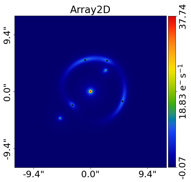
**PyAutoLens** has built in tools for modeling group-scale lenses, with no limit on the number of
lens and source galaxies!

Overviews of group and analysis are given in `notebooks/overview/overview_9_groups.ipynb`
The `autolens_workspace/*/group` package has example scripts for simulating datasets and lens modeling.


__Multi-Wavelength__

Modeling imaging datasets observed at different wavelengths (e.g. HST F814W and F150W) simultaneously or simultaneously
analysing imaging and interferometer data:

![g-band](https://raw.githubusercontent.com/PyAutoLabs/PyAutoLens/main/docs/overview/images/overview_3/g_image.png)

![r-band](https://raw.githubusercontent.com/PyAutoLabs/PyAutoLens/main/docs/overview/images/overview_3/r_image.png)

The appearance of the strong changes as a function of wavelength, therefore multi-wavelength analysis means we can learn
more about the different components in a galaxy (e.g a redder bulge and bluer disk) or when imaging and interferometer
data are combined, we can compare the emission from stars and dust.

Checkout the `autolens_workspace/*/multi` package to get started, however combining datasets is a more advanced
feature and it is recommended you first get to grips with the core API.


__Ellipse Fitting__

Ellipse fitting is a technique which fits many ellipses to a galaxy's emission to determine its ellipticity, position
angle and centre, without assuming a parametric form for its light (e.g. like a Seisc profile):

![ellipse](https://raw.githubusercontent.com/PyAutoLabs/PyAutoLens/main/docs/overview/images/overview_3/ellipse.png)

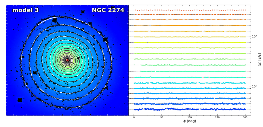
This provides complementary information to parametric light profile fitting, for example giving insights on whether
the ellipticity and position angle are constant with radius or if the galaxy's emission is lopsided. 

There are also multipole moment extensions to ellipse fitting, which determine higher order deviations from elliptical 
symmetry providing even more information on the galaxy's structure.

The following paper describes the technique in detail: https://arxiv.org/html/2407.12983v1

Checkout `autolens_workspace/notebooks/features/ellipse_fitting.ipynb` to learn how to use ellipse fitting.


__Shapelets__

Shapelets are a set of orthogonal basis functions that can be combined the represent galaxy structures:

Scientific Applications include capturing symmetric structures in a galaxy which are more complex than a Sersic profile,
irregular and asymmetric structures in a galaxy like spiral arms and providing a flexible model to deblend the emission 
of point sources (e.g. quasars) from the emission of their host galaxy.

Checkout `autolens_workspace/notebooks/features/shapelets.ipynb` to learn how to use shapelets.

__Operated Light Profiles__

An operated light profile is one where it is assumed to already be convolved with the PSF of the data, with the 
`Moffat` and `Gaussian` profiles common choices:

They are used for certain scientific applications where the PSF convolution is known to be a significant effect and
the knowledge of the PSF allows for detailed modeling abd deblending of the galaxy's light.

Checkout `autogalaxy_workspace/notebooks/features/operated_light_profiles.ipynb` to learn how to use operated profiles.

__Sky Background__

When an image of a galaxy is observed, the background sky contributes light to the image and adds noise:

For detailed studies of the outskirts of galaxies (e.g. stellar halos, faint extended disks), the sky background must be
accounted for in the model to ensure robust and accurate fits.

Checkout `autogalaxy_workspace/notebooks/features/sky_background.ipynb` to learn how to use include the sky
background in your model.


__Other:__

- mass models (aris paper)
- Automated pipelines / SLaM.
- Dark matter subhalos.
- Graphical models.
"""